可视化

这是原生可视化/编译器例子：当前 heatmap 要求 tg.Tensor，尚不接受 Torch Tensor。 安装 visualization extra；默认 CPU 可运行，选择 CUDA 时另需 cuda extra。 几何准备和编码不在编译器 IR 内，核心片段的初始化见折叠完整源码。

由场生成图像和视频：colormap 是编译出的 kernel， 几何光栅化（溅射、三角剖分）是 host 端的准备步骤，复用同一个颜色表达式； 视频导出经 Pillow（GIF 缓存全部帧）或 ffmpeg（MP4 逐帧流式编码）处理 raster。

• python examples/gpu_heatmap.py --device cpu --size 64 --output output/examples/heatmap.png
• python examples/visualize_fields.py --rings 8 --spokes 12 --steps 10 --size 128 --output output/examples
• python examples/visualize_mesh.py --model examples/assets/icosphere.obj --steps 2 --size 128 --output output/examples
• python examples/visualize_gaussians.py --count 100 --size 128 --output output/examples

运行后检查 output/examples/ 下的图像；MP4 导出额外依赖 ffmpeg。

GPU 热力图可视化准备

热力图把数字网格变成图像：每个数值映射为一种颜色。这里的 网格是取值在 [0, 1] 内的二维正弦图案；colormap 把每个标量 转换成红-绿-蓝（RGB）三元组，每个网格点对应一行像素数据。

\[ \mathrm{field}[y, x] = 0.5 + 0.5\,\sin\!\left(\tfrac{x}{17}\right) \cos\!\left(\tfrac{y}{23}\right) \]

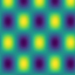
tg.visualize.heatmap 把广播算术和 colormap 组合成单个 “标量到 RGB”的 kernel。生成的 MLIR/provider 产物对外暴露， 可以直接查看；可选的 PNG 编码则留在编译器核心之外。

def scalar_field_to_rgb(size: int, device: str):
    values = [
        [0.5 + 0.5 * math.sin(x / 17.0) * math.cos(y / 23.0)
         for x in range(size)]
        for y in range(size)
    ]
    field = tg.tensor(values, dtype=tg.float32, device=device)  # (H, W)
    return tg.visualize.heatmap(field).realize()  # pixels (H*W, 3), viridis

默认 colormap 是内置的 viridis；cmap 切换到其他多停靠点 colormap—— 名称、RGB 颜色列表或 (position, RGB) 停靠点——low/high 则给出 朴素的双色 ramp，始终是同一个融合 kernel：

raster = tg.visualize.heatmap(field, cmap="magma")   # 名称见 tg.visualize.colormaps()

完整源码：examples/gpu_heatmap.py（可直接运行）

"""Compile a scalar field into RGB pixels and optionally save a PNG."""

from __future__ import annotations

import argparse
import math

import tiga as tg


def scalar_field_to_rgb(size: int, device: str):
    values = [
        [0.5 + 0.5 * math.sin(x / 17.0) * math.cos(y / 23.0)
         for x in range(size)]
        for y in range(size)
    ]
    field = tg.tensor(values, dtype=tg.float32, device=device)  # (H, W)
    return tg.visualize.heatmap(field).realize()  # pixels (H*W, 3), viridis


def main() -> None:
    parser = argparse.ArgumentParser()
    parser.add_argument("--device", default="cpu", choices=("cpu", "cuda"))
    parser.add_argument("--size", type=int, default=256)
    parser.add_argument("--output", default="output/examples/heatmap.png")
    args = parser.parse_args()

    raster = scalar_field_to_rgb(args.size, args.device)
    raster.save(args.output)

    # Inspect: raster.mlir(), raster.execution, raster.pixels.expression()


if __name__ == "__main__":
    main()

从位置出发的粒子与视频

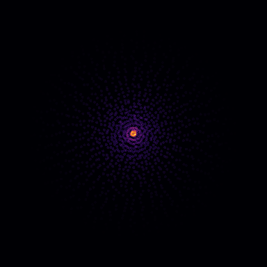
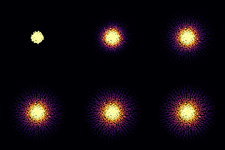
它是什么。 visualize_fields.py 跑了一个极简 FEM 式仿真：圆盘上的 稳态热传导，离散为带抖动的极坐标点集。核区（r ≤ 0.2）固定 T = 1， 外缘（r ≥ 0.95）固定 T = 0，每个内部节点向邻居均值松弛——即 拉普拉斯方程的 Jacobi 迭代，用 mean reducer 的 message passing 加 Dirichlet 掩码表达：

\[ T_i \leftarrow \frac{1}{|\mathcal{N}(i)|} \sum_{j \in \mathcal{N}(i)} T_j \;\; \text{（内部节点）}, \qquad T = 1 \;\text{于}\; \Gamma_{\mathrm{core}}, \quad T = 0 \;\text{于}\; \Gamma_{\mathrm{rim}} \]

邻居关系来自同一组点的 Delaunay 三角剖分，因此图与渲染网格严格一致。 每个节点渲染为一个圆盘，松弛过程由 tg.visualize.save_video 导出 为 GIF（host 缓存全部帧）或 MP4（逐帧流式编码）。

    tg.visualize.particles(                       # one disk per mesh node
        positions, values=snapshots[-1],
        width=args.size, height=args.size, point_radius=2.0,
        cmap="inferno",
    ).save(output / "fields_particles.png")

    frames = (                                    # generator: streamed, not buffered
        tg.visualize.particles(
            positions, values=T,
            width=256, height=256, point_radius=2.0,
            vmin=0.0, vmax=1.0, cmap="inferno")
        for T in snapshots[:: max(1, len(snapshots) // 24)]
    )
    tg.visualize.save_video(frames, output / "fields_diffusion.gif", fps=8)

完整源码：examples/visualize_fields.py（可直接运行）

"""Steady heat conduction on a disc: FEM-style mesh relaxation, rendered.

Shapes: positions (N, 2), temperature T (N,), boundary mask (N,),
raster pixels (H*W, 3). Outputs land in output/examples/.
"""

from __future__ import annotations

import argparse
from pathlib import Path

import numpy as np

import tiga as tg


class HeatRelax(tg.MessagePassing):
    """One Jacobi sweep for ∇²T = 0; Dirichlet nodes stay fixed."""

    reducer = tg.mean()

    def edge(self, src, dst, edge):
        return src.T

    def node(self, dst, flux):
        # boundary=1.0 keeps the prescribed temperature; interior relaxes
        return dst.boundary * dst.T + (1.0 - dst.boundary) * flux


def disc_points(rings: int, spokes: int, seed: int = 0):
    """Jittered polar grid on the unit disc: (N, 2) positions."""
    rng = np.random.default_rng(seed)
    radius = np.linspace(0.02, 1.0, rings)  # (R,)
    angle = np.linspace(0.0, 2.0 * np.pi, spokes, endpoint=False)  # (S,)
    r, a = np.meshgrid(radius, angle, indexing="ij")
    r = r + rng.uniform(-0.3, 0.3, r.shape) * (radius[1] - radius[0])
    a = a + rng.uniform(-0.3, 0.3, a.shape) * (angle[1] - angle[0])
    return np.stack([r.ravel() * np.cos(a.ravel()),
                     r.ravel() * np.sin(a.ravel())], axis=1)  # (N, 2)


def mesh_graph(faces: np.ndarray, num_vertices: int) -> tg.Graph:
    """Undirected vertex-adjacency CSR from the unique edges of ``faces``."""
    by_dst = [set() for _ in range(num_vertices)]
    for a, b, c in faces.tolist():
        for src, dst in ((a, b), (b, c), (c, a), (b, a), (c, b), (a, c)):
            by_dst[dst].add(src)
    row_ptr = np.zeros(num_vertices + 1, dtype=np.int64)
    col_idx: list[int] = []
    for dst, sources in enumerate(by_dst):
        col_idx.extend(sorted(sources))
        row_ptr[dst + 1] = len(col_idx)
    return tg.Graph.from_csr(
        tg.tensor(row_ptr.tolist(), dtype=tg.int64),  # (N+1,)
        tg.tensor(col_idx, dtype=tg.int64),           # (E,)
        num_src=num_vertices,
    )


def relax(positions: np.ndarray, boundary: np.ndarray, steps: int):
    from matplotlib.tri import Triangulation

    triangles = Triangulation(positions[:, 0], positions[:, 1]).triangles
    graph = mesh_graph(triangles, len(positions))
    kernel = HeatRelax()
    radius = np.hypot(positions[:, 0], positions[:, 1])  # (N,)
    temperature = np.where(radius <= 0.2, 1.0, 0.0)  # hot core, cold rim
    snapshots = [temperature]
    T = tg.tensor(temperature.tolist())       # (N,)
    fixed = tg.tensor(boundary.tolist())      # (N,)
    for _ in range(steps):
        T = kernel(graph=graph, ndata={"T": T, "boundary": fixed})  # (N,)
        snapshots.append(T.to_numpy())
        T = tg.tensor(snapshots[-1].tolist())
    return snapshots


def main() -> None:
    parser = argparse.ArgumentParser()
    parser.add_argument("--rings", type=int, default=28)
    parser.add_argument("--spokes", type=int, default=48)
    parser.add_argument("--steps", type=int, default=200)
    parser.add_argument("--size", type=int, default=384)
    parser.add_argument("--output", default="output/examples")
    args = parser.parse_args()

    positions = disc_points(args.rings, args.spokes)  # (N, 2)
    radius = np.hypot(positions[:, 0], positions[:, 1])
    boundary = ((radius <= 0.2) | (radius >= 0.95)).astype(np.float64)  # (N,)
    snapshots = relax(positions, boundary, steps=args.steps)
    output = Path(args.output)
    tg.visualize.particles(                       # one disk per mesh node
        positions, values=snapshots[-1],
        width=args.size, height=args.size, point_radius=2.0,
        cmap="inferno",
    ).save(output / "fields_particles.png")

    frames = (                                    # generator: streamed, not buffered
        tg.visualize.particles(
            positions, values=T,
            width=256, height=256, point_radius=2.0,
            vmin=0.0, vmax=1.0, cmap="inferno")
        for T in snapshots[:: max(1, len(snapshots) // 24)]
    )
    tg.visualize.save_video(frames, output / "fields_diffusion.gif", fps=8)

    tg.visualize.delaunay(                        # positions → faces: the FEM mesh
        positions, values=snapshots[-1],
        width=args.size, height=args.size,
        vmin=0.0, vmax=1.0, cmap="inferno",
    ).save(output / "fields_delaunay.png")

    # Inspect: raster.mlir(), tg.visualize.delaunay(...).execution


if __name__ == "__main__":
    main()

网格：从散点 Delaunay 或加载 OBJ

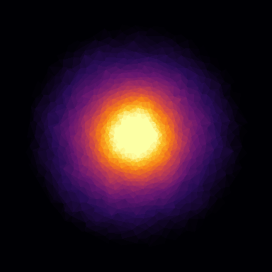
它是什么。 渲染连续表面需要 faces 而不只是 positions——faces 有两种 来源。仿真只给出离散位置时，由 Delaunay 三角剖分现算：tg.visualize.delaunay 把圆盘点集变成网格，每个三角形 按顶点值均值填充——稳态温度场由此呈现为经典的 FEM 云图。

    tg.visualize.delaunay(                        # positions → faces: the FEM mesh
        positions, values=snapshots[-1],
        width=args.size, height=args.size,
        vmin=0.0, vmax=1.0, cmap="inferno",
    ).save(output / "fields_delaunay.png")

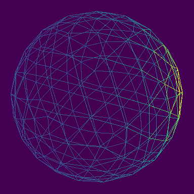
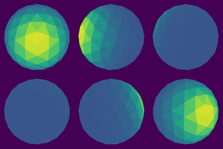
当三角剖分本身就是数据的一部分——求解器的表面网格、建模好的 3-D 模型——visualize_mesh.py 直接加载：用 tg.visualize.load_obj 从 OBJ 文件读入一个 细分 2 级的 icosphere（162 顶点、320 面），把无重复的网格边变成无向 Graph.from_csr 关系，并让一个高斯包从某个顶点出发经 mean reducer 扩散。随后同一 mesh 在固定 camera 下渲染，外加一段 12 帧 azimuth 环绕 导出的 GIF。

tg.visualize.mesh 直接使用给定的 faces——tg.visualize.delaunay 是从点现算三角剖分，mesh 则渲染仿真已经产出的三角形。重叠关系由 painter's algorithm 解决：三角形按顶点深度均值从远到近填充，球面近侧干净地遮挡远侧。 固定的 vmin/vmax 让各帧之间的颜色可比。

同一脚本还把几何体导出给 Blender 使用：tg.visualize.export_ply 写出 binary PLY，顶点同时携带扩散场的 顶点颜色与原始 scalar_value 属性；tg.visualize.export_obj 写出纯 positions/faces 文本格式，load_obj 可恒等读回。

    camera = tg.visualize.Camera.from_angles(
        25, -60, positions=positions)  # fixed elevation/azimuth view

    tg.visualize.mesh(                            # fill the given triangles
        positions, faces, values=u_render, camera=camera,
        width=args.size, height=args.size, vmin=0.0, vmax=vmax,
    ).save(output / "mesh_flat.png")
    tg.visualize.mesh(                            # same mesh as wireframe
        positions, faces, values=u_render, camera=camera,
        width=args.size, height=args.size, wireframe=True,
        vmin=0.0, vmax=vmax,
    ).save(output / "mesh_wireframe.png")
    tg.visualize.particles(                       # vertices splatted as disks
        positions, values=u_render, camera=camera,
        width=args.size, height=args.size, point_radius=2.0,
        vmin=0.0, vmax=vmax,
    ).save(output / "mesh_particles.png")

    frames = (                                    # 12-frame azimuth orbit
        tg.visualize.mesh(
            positions, faces, values=u_render,
            camera=tg.visualize.Camera.from_angles(
                25, azimuth, positions=positions),
            width=256, height=256, vmin=0.0, vmax=vmax)
        for azimuth in range(0, 360, 30)
    )
    tg.visualize.save_video(frames, output / "mesh_orbit.gif", fps=6)

    tg.visualize.export_ply(                      # Blender-ready binary dump
        output / "mesh.ply", positions, faces=faces, values=u_render)
    tg.visualize.export_obj(                      # geometry-only, load_obj-symmetric
        output / "mesh.obj", positions, faces)

完整源码：examples/visualize_mesh.py（可直接运行）

"""Diffuse a bump over an icosphere simulation mesh and render it.

Shapes: positions (N, 3), faces (M, 3), field u (N,), raster pixels
(H*W, 3). Outputs land in output/examples/.
"""

from __future__ import annotations

import argparse
from pathlib import Path

import numpy as np

import tiga as tg


class Diffusion(tg.MessagePassing):
    reducer = tg.mean()

    def edge(self, src, dst, edge):
        return src.u

    def node(self, dst, flux, rate):
        return dst.u + rate * (flux - dst.u)


def mesh_graph(faces: np.ndarray, num_vertices: int) -> tg.Graph:
    """Undirected vertex-adjacency CSR from the unique edges of ``faces``."""
    pairs = set()
    for a, b, c in faces.tolist():
        for src, dst in ((a, b), (b, c), (c, a)):
            pairs.add((src, dst))
            pairs.add((dst, src))
    by_dst = [[] for _ in range(num_vertices)]
    for src, dst in pairs:
        by_dst[dst].append(src)
    row_ptr = np.zeros(num_vertices + 1, dtype=np.int64)
    col_idx = []
    for dst, sources in enumerate(by_dst):
        col_idx.extend(sorted(sources))
        row_ptr[dst + 1] = len(col_idx)
    return tg.Graph.from_csr(
        tg.tensor(row_ptr.tolist(), dtype=tg.int64),  # (N+1,)
        tg.tensor(col_idx, dtype=tg.int64),           # (E,)
        num_src=num_vertices,
    )


def diffuse(graph: tg.Graph, u0: np.ndarray, steps: int, rate: float):
    kernel = Diffusion()
    u = tg.tensor(u0.tolist())  # (N,)
    for _ in range(steps):
        u = kernel(graph=graph, ndata={"u": u}, rate=rate)  # (N,)
        u = tg.tensor(u.to_numpy().tolist())
    return u.to_numpy()


def main() -> None:
    parser = argparse.ArgumentParser()
    parser.add_argument("--model", default="examples/assets/icosphere.obj")
    parser.add_argument("--steps", type=int, default=6)
    parser.add_argument("--size", type=int, default=384)
    parser.add_argument("--output", default="output/examples")
    args = parser.parse_args()

    positions, faces = tg.visualize.load_obj(args.model)  # (N, 3), (M, 3)
    graph = mesh_graph(faces, len(positions))
    direction = np.array([1.0, 0.0, 0.35])  # off-axis so the orbit reads
    top = positions[np.argmax(positions @ direction)]  # bump vertex (3,)
    u0 = np.exp(-(((positions - top) ** 2).sum(axis=1)) / 0.15)  # (N,)
    u = diffuse(graph, u0, steps=args.steps, rate=0.6)
    u_render = 0.12 + u  # ambient floor keeps the far side off the background
    vmax = float(u_render.max())  # fixed range: colors stay comparable

    output = Path(args.output)
    camera = tg.visualize.Camera.from_angles(
        25, -60, positions=positions)  # fixed elevation/azimuth view

    tg.visualize.mesh(                            # fill the given triangles
        positions, faces, values=u_render, camera=camera,
        width=args.size, height=args.size, vmin=0.0, vmax=vmax,
    ).save(output / "mesh_flat.png")
    tg.visualize.mesh(                            # same mesh as wireframe
        positions, faces, values=u_render, camera=camera,
        width=args.size, height=args.size, wireframe=True,
        vmin=0.0, vmax=vmax,
    ).save(output / "mesh_wireframe.png")
    tg.visualize.particles(                       # vertices splatted as disks
        positions, values=u_render, camera=camera,
        width=args.size, height=args.size, point_radius=2.0,
        vmin=0.0, vmax=vmax,
    ).save(output / "mesh_particles.png")

    frames = (                                    # 12-frame azimuth orbit
        tg.visualize.mesh(
            positions, faces, values=u_render,
            camera=tg.visualize.Camera.from_angles(
                25, azimuth, positions=positions),
            width=256, height=256, vmin=0.0, vmax=vmax)
        for azimuth in range(0, 360, 30)
    )
    tg.visualize.save_video(frames, output / "mesh_orbit.gif", fps=6)

    tg.visualize.export_ply(                      # Blender-ready binary dump
        output / "mesh.ply", positions, faces=faces, values=u_render)
    tg.visualize.export_obj(                      # geometry-only, load_obj-symmetric
        output / "mesh.obj", positions, faces)

    # Inspect: camera.world_to_ndc(positions), raster.mlir()


if __name__ == "__main__":
    main()

Gaussian splats 与体渲染

同一组 3-D Gaussian，两种观察方式： tg.visualize.gaussians 展示每个 Gaussian 的颜色与形状； tg.visualize.volume 展示它们在空间中叠加形成的密度。

Gaussian splats
直接合成带颜色的椭圆足迹。

Volume
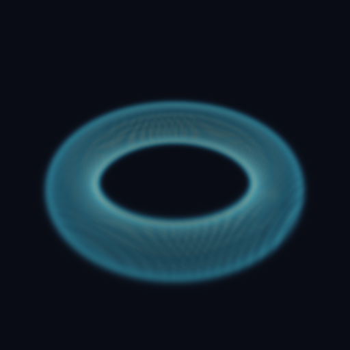
采样密度网格，沿视线累积颜色与吸收。

这是可复现的合成场景，不是从照片训练的模型。圆环由 2,200 个 Gaussian 组成，两图共用相机与位置；左图的 RGB 预先加入了固定光照，右图按密度着色， 因此不是像素级等价对照。渲染与投影当前由 host NumPy 执行，不是 GPU 渲染 benchmark。

渲染 Gaussian

positions、colors 和 scales 均为 (N, 3) 数组；rotations 是 (N, 4) 的 (w, x, y, z) quaternion，opacities 是 (N,)。 本例的长轴沿圆环切向排列，scales 给出三个主轴的标准差。

    camera = tg.visualize.Camera.from_angles(38, -55, distance=2.6)

    tg.visualize.gaussians(
        positions, colors, scales,
        rotations=rotations, opacities=opacities, camera=camera,
        width=args.size, height=args.size, background=background,
    ).save(output / "gaussians_splats.png")

positions 等场景数组由脚本中的 torus_gaussians 生成； args.size、output 来自命令行，background 为深蓝灰色 RGB。 完整初始化见下方源码。两种输出均为 Raster，通过 .save() 写出 PNG。

同一场景改用体渲染

splat_density 是这个示例的辅助函数：把切向 Gaussian 的各向异性密度采样到 64 × 64 × 64 网格，覆盖 [-1, 1]³。它不保留逐 Gaussian 的 RGB； cmap 重新按密度着色。相机与上方完全一致。

    density = splat_density(positions, opacities, scales)
    tg.visualize.volume(
        density, camera=camera, width=args.size, height=args.size,
        cmap=[(0.10, 0.18, 0.30), (0.20, 0.62, 0.72), (0.96, 0.83, 0.60)],
        scale=4.0, background=background,
    ).save(output / "gaussians_volume.png")

旋转查看

固定仰角，相机环绕一周。36 帧、12 fps；点击播放，不自动播放。

复现本页图片与视频（MP4 编码需要 ffmpeg）：

python examples/visualize_gaussians.py --count 2200 --size 512 --frames 36 --video-format mp4 --output output/examples

默认使用固定随机种子。省略 --video-format mp4 时导出 GIF；渲染不需要 ffmpeg。

完整源码：examples/visualize_gaussians.py

"""Render an anisotropic Gaussian scene two ways: splats and volume.

Shapes: positions (N, 3), colors (N, 3), scales (N, 3), rotations (N, 4),
density grid (X, Y, Z), raster pixels (H*W, 3). Outputs land in
output/examples/.
"""

from __future__ import annotations

import argparse
from pathlib import Path

import numpy as np

import tiga as tg


def torus_gaussians(count: int, seed: int = 0):
    """Colored Gaussians on a torus, stretched along the tangent."""
    if count < 1:
        raise ValueError("count must be positive")
    rng = np.random.default_rng(seed)
    # Stratified angles avoid gaps while retaining a seeded, irregular cloud.
    angle = (np.arange(count) + rng.random(count)) * (2.0 * np.pi / count)
    tube_angle = (np.arange(count) * np.pi * (3.0 - np.sqrt(5.0)) + rng.uniform(0, 2*np.pi)) % (2*np.pi)
    tube_radius = 0.14
    ring = 0.62 + tube_radius * np.cos(tube_angle)
    positions = np.stack([ring * np.cos(angle), ring * np.sin(angle),
                          tube_radius * np.sin(tube_angle)], axis=1)  # (N, 3)
    # A proper z rotation maps local x onto the torus tangent. Using
    # (tangent, outward radial, vertical) as columns would be a reflection.
    half_angle = (angle + np.pi / 2.0) / 2.0
    rotations = np.stack([np.cos(half_angle), np.zeros(count),
                          np.zeros(count), np.sin(half_angle)], axis=1)
    scales = np.broadcast_to([0.035, 0.018, 0.018], (count, 3)).copy()
    # One restrained cool-to-warm sweep; position, not density, sets this RGB.
    blend = (0.5 + 0.5 * np.cos(angle - 0.5))[:, None]
    colors = (1.0 - blend) * np.array([0.20, 0.55, 0.70]) + blend * np.array([0.93, 0.66, 0.38])
    normals = np.stack([np.cos(angle) * np.cos(tube_angle),
                        np.sin(angle) * np.cos(tube_angle), np.sin(tube_angle)], axis=1)
    light = np.array([0.3, -0.4, 0.85])
    diffuse = np.maximum(normals @ (light / np.linalg.norm(light)), 0)[:, None]
    # Bake a fixed light into RGB; the renderer itself does not shade normals.
    colors = np.clip(colors * (0.35 + 0.65 * diffuse) + 0.12 * diffuse**10, 0, 1)
    opacities = np.full(count, 0.75)
    return positions, colors, scales, rotations, opacities


def splat_density(positions: np.ndarray, opacities: np.ndarray,
                  scales: np.ndarray, voxel: int = 64):
    """Sample this scene's tangent-aligned Gaussians on the unit cube.

    The volume retains the anisotropic density, not the per-Gaussian RGB.
    Each contribution is truncated at a three-sigma bounding box.
    """
    if voxel < 2:
        raise ValueError("voxel must be at least 2")
    grid = np.zeros((voxel, voxel, voxel))
    for position, opacity, sigma in zip(positions, opacities, scales, strict=True):
        center = (position + 1.0) * 0.5 * (voxel - 1)
        radius = 3.0 * max(sigma) * 0.5 * (voxel - 1)
        lo = np.maximum(np.floor(center - radius).astype(int), 0)
        hi = np.minimum(np.ceil(center + radius).astype(int) + 1, voxel)
        axes = [np.arange(lo[d], hi[d]) for d in range(3)]
        if any(len(axis) == 0 for axis in axes):
            continue
        gx, gy, gz = np.meshgrid(*axes, indexing="ij")
        dx, dy, dz = [(axis - c) * 2.0 / (voxel - 1)
                      for axis, c in zip((gx, gy, gz), center)]
        angle = np.arctan2(position[1], position[0])
        along = -np.sin(angle) * dx + np.cos(angle) * dy
        across = np.cos(angle) * dx + np.sin(angle) * dy
        distance2 = (along / sigma[0])**2 + (across / sigma[1])**2 + (dz / sigma[2])**2
        grid[lo[0]:hi[0], lo[1]:hi[1], lo[2]:hi[2]] += (
            opacity * np.exp(-0.5 * distance2))
    return grid  # (X, Y, Z)


def main() -> None:
    parser = argparse.ArgumentParser()
    parser.add_argument("--count", type=int, default=2200)
    parser.add_argument("--size", type=int, default=512)
    parser.add_argument("--frames", type=int, default=36)
    parser.add_argument("--video-format", choices=("gif", "mp4"), default="gif")
    parser.add_argument("--output", default="output/examples")
    args = parser.parse_args()
    if min(args.count, args.size, args.frames) < 1:
        parser.error("count, size and frames must be positive")

    positions, colors, scales, rotations, opacities = torus_gaussians(
        args.count)
    output = Path(args.output)
    background = (0.035, 0.048, 0.08)
    camera = tg.visualize.Camera.from_angles(38, -55, distance=2.6)

    tg.visualize.gaussians(
        positions, colors, scales,
        rotations=rotations, opacities=opacities, camera=camera,
        width=args.size, height=args.size, background=background,
    ).save(output / "gaussians_splats.png")

    density = splat_density(positions, opacities, scales)
    tg.visualize.volume(
        density, camera=camera, width=args.size, height=args.size,
        cmap=[(0.10, 0.18, 0.30), (0.20, 0.62, 0.72), (0.96, 0.83, 0.60)],
        scale=4.0, background=background,
    ).save(output / "gaussians_volume.png")

    frames = (
        tg.visualize.gaussians(
            positions, colors, scales,
            rotations=rotations, opacities=opacities,
            camera=tg.visualize.Camera.from_angles(
                38, azimuth, distance=2.6),
            width=384, height=384, background=background)
        for azimuth in np.linspace(-55, 305, args.frames, endpoint=False)
    )
    tg.visualize.save_video(frames, output / f"gaussians_orbit.{args.video_format}", fps=12)

    # Inspect: camera.world_to_ndc(positions), raster.to_numpy()


if __name__ == "__main__":
    main()

渲染原理：投影、遮挡与密度

一个 Gaussian 由中心、方向和三个轴向尺度定义。旋转矩阵为 R 时，其协方差为：

\[ \Sigma = R\,\mathrm{diag}(s^2)\,R^\top \]

透视投影的 Jacobian 将其变为屏幕上的二维椭圆。令像素距椭圆中心的偏移为 δ，投影协方差为 Σ′，不透明度为 oᵢ，则：

\[ \alpha_i = o_i \exp\!\left(-\tfrac12\delta^\top\Sigma'^{-1}\delta\right) \]

Gaussian 按中心深度从近到远处理。transmittance 表示前面各层之后剩余的透射率； 最终颜色包含未被遮挡的背景：

\[ T_i = \prod_{j<i}(1-\alpha_j),\qquad C = \sum_i T_i\alpha_i c_i + T_{\mathrm{end}}c_{\mathrm{background}} \]

体渲染改为沿每条视线采样密度。每一步的不透明度由采样密度、scale 与步长决定：

\[ \alpha = 1-\exp(-\sigma\,\mathrm{scale}\,\Delta t) \]

从训练结果导入 Gaussian

tg.visualize.load_ply 返回位置、可选 faces 和附加属性。常见 3DGS PLY 将颜色 DC 系数存在 f_dc_*，旋转存在 rot_*，并保存未经激活的 opacity 与 log-scale。 对这种布局，转换关系为：

\[ \mathrm{RGB}=\mathrm{clip}(0.5+0.2821\,f_{\mathrm{dc}},0,1) \]

\[ o=\mathrm{sigmoid}(\mathrm{opacity}),\qquad s=\exp(\mathrm{scale}) \]

按编号顺序堆叠各属性后，传给 tg.visualize.gaussians。 这是仅使用 DC 颜色的显示方式，不求值高阶、随视角变化的 spherical harmonics； 不同导出工具的属性约定应先核对。