Visualization

These are native visualization/compiler examples: heatmap currently requires tg.Tensor, not a Torch tensor. Install the visualization extra; CPU is the default, and CUDA additionally needs the cuda extra. Geometry preparation and encoding are outside compiler IR; expanded full sources include snippet setup.

Fields become images and videos: the colormap is a compiled kernel, geometry rasterization (splat, triangulation) is a host-side preparation feeding the same color expression, and video export encodes rasters through Pillow (GIF buffers all frames) or ffmpeg (MP4 streams frames).

• python examples/gpu_heatmap.py --device cpu --size 64 --output output/examples/heatmap.png
• python examples/visualize_fields.py --rings 8 --spokes 12 --steps 10 --size 128 --output output/examples
• python examples/visualize_mesh.py --model examples/assets/icosphere.obj --steps 2 --size 128 --output output/examples
• python examples/visualize_gaussians.py --count 100 --size 128 --output output/examples

Inspect the images under output/examples/; MP4 export additionally requires ffmpeg.

GPU heatmap visualization prep

A heatmap turns a grid of numbers into an image by mapping each value to a color. Here the grid is a two-dimensional sinusoidal pattern with values in [0, 1]; a colormap converts every scalar into a red-green-blue (RGB) triple, yielding one row of pixel data per grid point.

\[ \mathrm{field}[y, x] = 0.5 + 0.5\,\sin\!\left(\tfrac{x}{17}\right) \cos\!\left(\tfrac{y}{23}\right) \]

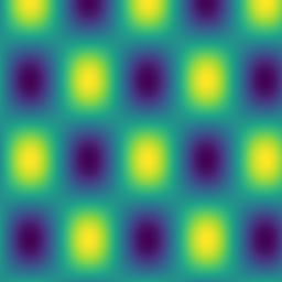
tg.visualize.heatmap composes the broadcast arithmetic and the colormap into a single scalar-to-RGB kernel. The generated MLIR/provider artifact is exposed for inspection, and the optional PNG encoding stays outside the compiler core.

def scalar_field_to_rgb(size: int, device: str):
    values = [
        [0.5 + 0.5 * math.sin(x / 17.0) * math.cos(y / 23.0)
         for x in range(size)]
        for y in range(size)
    ]
    field = tg.tensor(values, dtype=tg.float32, device=device)  # (H, W)
    return tg.visualize.heatmap(field).realize()  # pixels (H*W, 3), viridis

The default colormap is the built-in viridis; cmap switches to another multi-stop colormap — a name, a list of RGB colors, or (position, RGB) stops — and low/high give a plain two-color ramp, always in the same fused kernel:

raster = tg.visualize.heatmap(field, cmap="magma")   # see tg.visualize.colormaps()

Full source: examples/gpu_heatmap.py (runs as-is)

"""Compile a scalar field into RGB pixels and optionally save a PNG."""

from __future__ import annotations

import argparse
import math

import tiga as tg


def scalar_field_to_rgb(size: int, device: str):
    values = [
        [0.5 + 0.5 * math.sin(x / 17.0) * math.cos(y / 23.0)
         for x in range(size)]
        for y in range(size)
    ]
    field = tg.tensor(values, dtype=tg.float32, device=device)  # (H, W)
    return tg.visualize.heatmap(field).realize()  # pixels (H*W, 3), viridis


def main() -> None:
    parser = argparse.ArgumentParser()
    parser.add_argument("--device", default="cpu", choices=("cpu", "cuda"))
    parser.add_argument("--size", type=int, default=256)
    parser.add_argument("--output", default="output/examples/heatmap.png")
    args = parser.parse_args()

    raster = scalar_field_to_rgb(args.size, args.device)
    raster.save(args.output)

    # Inspect: raster.mlir(), raster.execution, raster.pixels.expression()


if __name__ == "__main__":
    main()

Particles and video from positions

What it is. visualize_fields.py runs a tiny FEM-style simulation: steady heat conduction on a disc, discretized as a jittered polar point set. The core (r ≤ 0.2) is held at T = 1 and the rim (r ≥ 0.95) at T = 0; every interior node relaxes toward its neighbor mean — a Jacobi sweep for the Laplace equation, expressed as message passing with a mean reducer and a Dirichlet mask:

\[ T_i \leftarrow \frac{1}{|\mathcal{N}(i)|} \sum_{j \in \mathcal{N}(i)} T_j \;\; \text{(interior)}, \qquad T = 1 \;\text{on}\; \Gamma_{\mathrm{core}}, \quad T = 0 \;\text{on}\; \Gamma_{\mathrm{rim}} \]

The neighbor relation comes from the Delaunay triangulation of the same points, so the graph and the rendered mesh agree exactly. Each node renders as one disk splat, and tg.visualize.save_video exports the relaxation into a GIF (host-buffered) or MP4 (streamed).

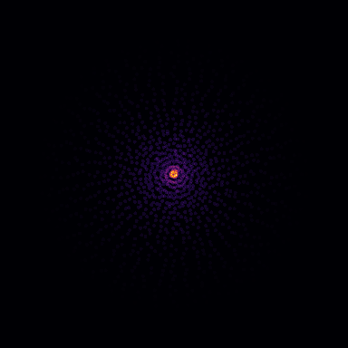
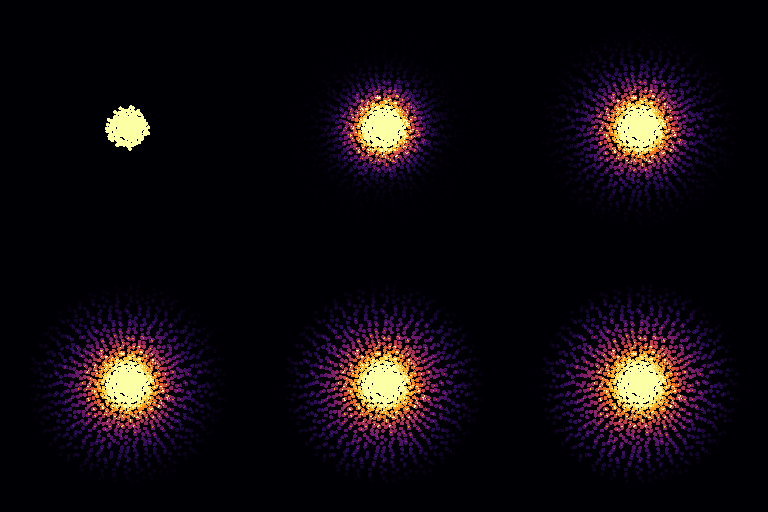
    tg.visualize.particles(                       # one disk per mesh node
        positions, values=snapshots[-1],
        width=args.size, height=args.size, point_radius=2.0,
        cmap="inferno",
    ).save(output / "fields_particles.png")

    frames = (                                    # generator: streamed, not buffered
        tg.visualize.particles(
            positions, values=T,
            width=256, height=256, point_radius=2.0,
            vmin=0.0, vmax=1.0, cmap="inferno")
        for T in snapshots[:: max(1, len(snapshots) // 24)]
    )
    tg.visualize.save_video(frames, output / "fields_diffusion.gif", fps=8)

Full source: examples/visualize_fields.py (runs as-is)

"""Steady heat conduction on a disc: FEM-style mesh relaxation, rendered.

Shapes: positions (N, 2), temperature T (N,), boundary mask (N,),
raster pixels (H*W, 3). Outputs land in output/examples/.
"""

from __future__ import annotations

import argparse
from pathlib import Path

import numpy as np

import tiga as tg


class HeatRelax(tg.MessagePassing):
    """One Jacobi sweep for ∇²T = 0; Dirichlet nodes stay fixed."""

    reducer = tg.mean()

    def edge(self, src, dst, edge):
        return src.T

    def node(self, dst, flux):
        # boundary=1.0 keeps the prescribed temperature; interior relaxes
        return dst.boundary * dst.T + (1.0 - dst.boundary) * flux


def disc_points(rings: int, spokes: int, seed: int = 0):
    """Jittered polar grid on the unit disc: (N, 2) positions."""
    rng = np.random.default_rng(seed)
    radius = np.linspace(0.02, 1.0, rings)  # (R,)
    angle = np.linspace(0.0, 2.0 * np.pi, spokes, endpoint=False)  # (S,)
    r, a = np.meshgrid(radius, angle, indexing="ij")
    r = r + rng.uniform(-0.3, 0.3, r.shape) * (radius[1] - radius[0])
    a = a + rng.uniform(-0.3, 0.3, a.shape) * (angle[1] - angle[0])
    return np.stack([r.ravel() * np.cos(a.ravel()),
                     r.ravel() * np.sin(a.ravel())], axis=1)  # (N, 2)


def mesh_graph(faces: np.ndarray, num_vertices: int) -> tg.Graph:
    """Undirected vertex-adjacency CSR from the unique edges of ``faces``."""
    by_dst = [set() for _ in range(num_vertices)]
    for a, b, c in faces.tolist():
        for src, dst in ((a, b), (b, c), (c, a), (b, a), (c, b), (a, c)):
            by_dst[dst].add(src)
    row_ptr = np.zeros(num_vertices + 1, dtype=np.int64)
    col_idx: list[int] = []
    for dst, sources in enumerate(by_dst):
        col_idx.extend(sorted(sources))
        row_ptr[dst + 1] = len(col_idx)
    return tg.Graph.from_csr(
        tg.tensor(row_ptr.tolist(), dtype=tg.int64),  # (N+1,)
        tg.tensor(col_idx, dtype=tg.int64),           # (E,)
        num_src=num_vertices,
    )


def relax(positions: np.ndarray, boundary: np.ndarray, steps: int):
    from matplotlib.tri import Triangulation

    triangles = Triangulation(positions[:, 0], positions[:, 1]).triangles
    graph = mesh_graph(triangles, len(positions))
    kernel = HeatRelax()
    radius = np.hypot(positions[:, 0], positions[:, 1])  # (N,)
    temperature = np.where(radius <= 0.2, 1.0, 0.0)  # hot core, cold rim
    snapshots = [temperature]
    T = tg.tensor(temperature.tolist())       # (N,)
    fixed = tg.tensor(boundary.tolist())      # (N,)
    for _ in range(steps):
        T = kernel(graph=graph, ndata={"T": T, "boundary": fixed})  # (N,)
        snapshots.append(T.to_numpy())
        T = tg.tensor(snapshots[-1].tolist())
    return snapshots


def main() -> None:
    parser = argparse.ArgumentParser()
    parser.add_argument("--rings", type=int, default=28)
    parser.add_argument("--spokes", type=int, default=48)
    parser.add_argument("--steps", type=int, default=200)
    parser.add_argument("--size", type=int, default=384)
    parser.add_argument("--output", default="output/examples")
    args = parser.parse_args()

    positions = disc_points(args.rings, args.spokes)  # (N, 2)
    radius = np.hypot(positions[:, 0], positions[:, 1])
    boundary = ((radius <= 0.2) | (radius >= 0.95)).astype(np.float64)  # (N,)
    snapshots = relax(positions, boundary, steps=args.steps)
    output = Path(args.output)
    tg.visualize.particles(                       # one disk per mesh node
        positions, values=snapshots[-1],
        width=args.size, height=args.size, point_radius=2.0,
        cmap="inferno",
    ).save(output / "fields_particles.png")

    frames = (                                    # generator: streamed, not buffered
        tg.visualize.particles(
            positions, values=T,
            width=256, height=256, point_radius=2.0,
            vmin=0.0, vmax=1.0, cmap="inferno")
        for T in snapshots[:: max(1, len(snapshots) // 24)]
    )
    tg.visualize.save_video(frames, output / "fields_diffusion.gif", fps=8)

    tg.visualize.delaunay(                        # positions → faces: the FEM mesh
        positions, values=snapshots[-1],
        width=args.size, height=args.size,
        vmin=0.0, vmax=1.0, cmap="inferno",
    ).save(output / "fields_delaunay.png")

    # Inspect: raster.mlir(), tg.visualize.delaunay(...).execution


if __name__ == "__main__":
    main()

Meshes: Delaunay from points or loaded OBJ

What it is. Rendering a continuous surface needs faces, not just positions — and faces arrive two ways. When a simulation produces only scattered positions, Delaunay triangulation computes them: tg.visualize.delaunay turns the disc's point set into a mesh and fills each triangle with its mean vertex value — the steady temperature field drawn as a classic FEM contour plot.

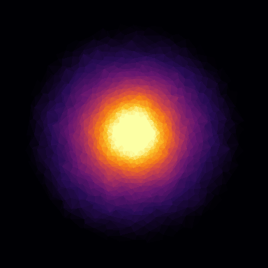
    tg.visualize.delaunay(                        # positions → faces: the FEM mesh
        positions, values=snapshots[-1],
        width=args.size, height=args.size,
        vmin=0.0, vmax=1.0, cmap="inferno",
    ).save(output / "fields_delaunay.png")

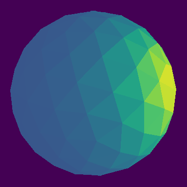
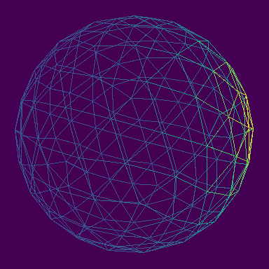
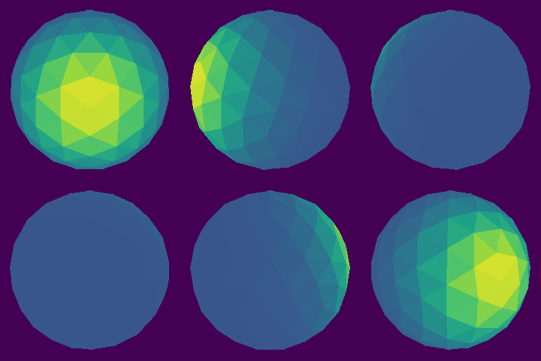
When the triangulation is part of the data — a solver's surface mesh, a sculpted 3-D model — visualize_mesh.py loads it directly: a subdivision-2 icosphere (162 vertices, 320 faces) from an OBJ file via tg.visualize.load_obj, its unique mesh edges turned into an undirected Graph.from_csr relation, a Gaussian bump diffused from one vertex through a mean reducer. The mesh then renders from a fixed camera, plus a twelve-frame azimuth orbit exported as GIF.

tg.visualize.mesh takes the faces as given — where tg.visualize.delaunay computes a triangulation from points, mesh renders the triangles a simulation already produced. Overlap resolves through the painter's algorithm: triangles fill far-to-near by mean vertex depth, so the near side of the sphere cleanly occludes the far side. A fixed vmin/vmax keeps the colors comparable across orbit frames.

The same script also exports the geometry for Blender: tg.visualize.export_ply writes a binary PLY whose vertices carry the diffused field both as vertex colors and as a raw scalar_value attribute, and tg.visualize.export_obj writes the plain positions/faces text format that load_obj reads back identically.

    camera = tg.visualize.Camera.from_angles(
        25, -60, positions=positions)  # fixed elevation/azimuth view

    tg.visualize.mesh(                            # fill the given triangles
        positions, faces, values=u_render, camera=camera,
        width=args.size, height=args.size, vmin=0.0, vmax=vmax,
    ).save(output / "mesh_flat.png")
    tg.visualize.mesh(                            # same mesh as wireframe
        positions, faces, values=u_render, camera=camera,
        width=args.size, height=args.size, wireframe=True,
        vmin=0.0, vmax=vmax,
    ).save(output / "mesh_wireframe.png")
    tg.visualize.particles(                       # vertices splatted as disks
        positions, values=u_render, camera=camera,
        width=args.size, height=args.size, point_radius=2.0,
        vmin=0.0, vmax=vmax,
    ).save(output / "mesh_particles.png")

    frames = (                                    # 12-frame azimuth orbit
        tg.visualize.mesh(
            positions, faces, values=u_render,
            camera=tg.visualize.Camera.from_angles(
                25, azimuth, positions=positions),
            width=256, height=256, vmin=0.0, vmax=vmax)
        for azimuth in range(0, 360, 30)
    )
    tg.visualize.save_video(frames, output / "mesh_orbit.gif", fps=6)

    tg.visualize.export_ply(                      # Blender-ready binary dump
        output / "mesh.ply", positions, faces=faces, values=u_render)
    tg.visualize.export_obj(                      # geometry-only, load_obj-symmetric
        output / "mesh.obj", positions, faces)

Full source: examples/visualize_mesh.py (runs as-is)

"""Diffuse a bump over an icosphere simulation mesh and render it.

Shapes: positions (N, 3), faces (M, 3), field u (N,), raster pixels
(H*W, 3). Outputs land in output/examples/.
"""

from __future__ import annotations

import argparse
from pathlib import Path

import numpy as np

import tiga as tg


class Diffusion(tg.MessagePassing):
    reducer = tg.mean()

    def edge(self, src, dst, edge):
        return src.u

    def node(self, dst, flux, rate):
        return dst.u + rate * (flux - dst.u)


def mesh_graph(faces: np.ndarray, num_vertices: int) -> tg.Graph:
    """Undirected vertex-adjacency CSR from the unique edges of ``faces``."""
    pairs = set()
    for a, b, c in faces.tolist():
        for src, dst in ((a, b), (b, c), (c, a)):
            pairs.add((src, dst))
            pairs.add((dst, src))
    by_dst = [[] for _ in range(num_vertices)]
    for src, dst in pairs:
        by_dst[dst].append(src)
    row_ptr = np.zeros(num_vertices + 1, dtype=np.int64)
    col_idx = []
    for dst, sources in enumerate(by_dst):
        col_idx.extend(sorted(sources))
        row_ptr[dst + 1] = len(col_idx)
    return tg.Graph.from_csr(
        tg.tensor(row_ptr.tolist(), dtype=tg.int64),  # (N+1,)
        tg.tensor(col_idx, dtype=tg.int64),           # (E,)
        num_src=num_vertices,
    )


def diffuse(graph: tg.Graph, u0: np.ndarray, steps: int, rate: float):
    kernel = Diffusion()
    u = tg.tensor(u0.tolist())  # (N,)
    for _ in range(steps):
        u = kernel(graph=graph, ndata={"u": u}, rate=rate)  # (N,)
        u = tg.tensor(u.to_numpy().tolist())
    return u.to_numpy()


def main() -> None:
    parser = argparse.ArgumentParser()
    parser.add_argument("--model", default="examples/assets/icosphere.obj")
    parser.add_argument("--steps", type=int, default=6)
    parser.add_argument("--size", type=int, default=384)
    parser.add_argument("--output", default="output/examples")
    args = parser.parse_args()

    positions, faces = tg.visualize.load_obj(args.model)  # (N, 3), (M, 3)
    graph = mesh_graph(faces, len(positions))
    direction = np.array([1.0, 0.0, 0.35])  # off-axis so the orbit reads
    top = positions[np.argmax(positions @ direction)]  # bump vertex (3,)
    u0 = np.exp(-(((positions - top) ** 2).sum(axis=1)) / 0.15)  # (N,)
    u = diffuse(graph, u0, steps=args.steps, rate=0.6)
    u_render = 0.12 + u  # ambient floor keeps the far side off the background
    vmax = float(u_render.max())  # fixed range: colors stay comparable

    output = Path(args.output)
    camera = tg.visualize.Camera.from_angles(
        25, -60, positions=positions)  # fixed elevation/azimuth view

    tg.visualize.mesh(                            # fill the given triangles
        positions, faces, values=u_render, camera=camera,
        width=args.size, height=args.size, vmin=0.0, vmax=vmax,
    ).save(output / "mesh_flat.png")
    tg.visualize.mesh(                            # same mesh as wireframe
        positions, faces, values=u_render, camera=camera,
        width=args.size, height=args.size, wireframe=True,
        vmin=0.0, vmax=vmax,
    ).save(output / "mesh_wireframe.png")
    tg.visualize.particles(                       # vertices splatted as disks
        positions, values=u_render, camera=camera,
        width=args.size, height=args.size, point_radius=2.0,
        vmin=0.0, vmax=vmax,
    ).save(output / "mesh_particles.png")

    frames = (                                    # 12-frame azimuth orbit
        tg.visualize.mesh(
            positions, faces, values=u_render,
            camera=tg.visualize.Camera.from_angles(
                25, azimuth, positions=positions),
            width=256, height=256, vmin=0.0, vmax=vmax)
        for azimuth in range(0, 360, 30)
    )
    tg.visualize.save_video(frames, output / "mesh_orbit.gif", fps=6)

    tg.visualize.export_ply(                      # Blender-ready binary dump
        output / "mesh.ply", positions, faces=faces, values=u_render)
    tg.visualize.export_obj(                      # geometry-only, load_obj-symmetric
        output / "mesh.obj", positions, faces)

    # Inspect: camera.world_to_ndc(positions), raster.mlir()


if __name__ == "__main__":
    main()

Gaussian splats and volumes

One set of 3-D Gaussians, two views: tg.visualize.gaussians shows their individual colors and shapes; tg.visualize.volume shows the density they accumulate in space.

Gaussian splats
Composite the colored elliptical footprints directly.

Volume
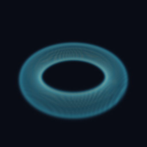
Sample density and accumulate emission and absorption along each ray.

This reproducible synthetic scene contains 2,200 Gaussians, not a model trained from photographs. Both images share positions and camera. The left image has fixed lighting baked into its RGB; the right maps density to color, so this is not a pixel-equivalence comparison. Projection and rendering currently run in host NumPy; this is not a GPU rendering benchmark.

Render Gaussians

positions, colors and scales are (N, 3) arrays; rotations contains (N, 4) quaternions in (w, x, y, z) order, and opacities is (N,). The long axes follow the ring tangent; scales specifies standard deviations along the three principal axes.

    camera = tg.visualize.Camera.from_angles(38, -55, distance=2.6)

    tg.visualize.gaussians(
        positions, colors, scales,
        rotations=rotations, opacities=opacities, camera=camera,
        width=args.size, height=args.size, background=background,
    ).save(output / "gaussians_splats.png")

The script's torus_gaussians helper creates the scene arrays. args.size and output come from the command line; background is a dark blue-gray RGB value. Complete initialization appears in the source below. Both renderers return a Raster whose .save() method writes PNG.

Render the same scene as a volume

The example-specific splat_density helper samples the tangent-aligned, anisotropic density into a 64 × 64 × 64 grid spanning [-1, 1]³. Individual RGB values are not retained: cmap colors the density instead. The camera is unchanged.

    density = splat_density(positions, opacities, scales)
    tg.visualize.volume(
        density, camera=camera, width=args.size, height=args.size,
        cmap=[(0.10, 0.18, 0.30), (0.20, 0.62, 0.72), (0.96, 0.83, 0.60)],
        scale=4.0, background=background,
    ).save(output / "gaussians_volume.png")

Orbit the scene

One orbit at a fixed elevation. 36 frames at 12 fps; play on demand, with no autoplay.

Reproduce the images and video (MP4 encoding requires ffmpeg):

python examples/visualize_gaussians.py --count 2200 --size 512 --frames 36 --video-format mp4 --output output/examples

The random seed is fixed. Omit --video-format mp4 to export GIF instead; rendering itself does not require ffmpeg.

Full source: examples/visualize_gaussians.py

"""Render an anisotropic Gaussian scene two ways: splats and volume.

Shapes: positions (N, 3), colors (N, 3), scales (N, 3), rotations (N, 4),
density grid (X, Y, Z), raster pixels (H*W, 3). Outputs land in
output/examples/.
"""

from __future__ import annotations

import argparse
from pathlib import Path

import numpy as np

import tiga as tg


def torus_gaussians(count: int, seed: int = 0):
    """Colored Gaussians on a torus, stretched along the tangent."""
    if count < 1:
        raise ValueError("count must be positive")
    rng = np.random.default_rng(seed)
    # Stratified angles avoid gaps while retaining a seeded, irregular cloud.
    angle = (np.arange(count) + rng.random(count)) * (2.0 * np.pi / count)
    tube_angle = (np.arange(count) * np.pi * (3.0 - np.sqrt(5.0)) + rng.uniform(0, 2*np.pi)) % (2*np.pi)
    tube_radius = 0.14
    ring = 0.62 + tube_radius * np.cos(tube_angle)
    positions = np.stack([ring * np.cos(angle), ring * np.sin(angle),
                          tube_radius * np.sin(tube_angle)], axis=1)  # (N, 3)
    # A proper z rotation maps local x onto the torus tangent. Using
    # (tangent, outward radial, vertical) as columns would be a reflection.
    half_angle = (angle + np.pi / 2.0) / 2.0
    rotations = np.stack([np.cos(half_angle), np.zeros(count),
                          np.zeros(count), np.sin(half_angle)], axis=1)
    scales = np.broadcast_to([0.035, 0.018, 0.018], (count, 3)).copy()
    # One restrained cool-to-warm sweep; position, not density, sets this RGB.
    blend = (0.5 + 0.5 * np.cos(angle - 0.5))[:, None]
    colors = (1.0 - blend) * np.array([0.20, 0.55, 0.70]) + blend * np.array([0.93, 0.66, 0.38])
    normals = np.stack([np.cos(angle) * np.cos(tube_angle),
                        np.sin(angle) * np.cos(tube_angle), np.sin(tube_angle)], axis=1)
    light = np.array([0.3, -0.4, 0.85])
    diffuse = np.maximum(normals @ (light / np.linalg.norm(light)), 0)[:, None]
    # Bake a fixed light into RGB; the renderer itself does not shade normals.
    colors = np.clip(colors * (0.35 + 0.65 * diffuse) + 0.12 * diffuse**10, 0, 1)
    opacities = np.full(count, 0.75)
    return positions, colors, scales, rotations, opacities


def splat_density(positions: np.ndarray, opacities: np.ndarray,
                  scales: np.ndarray, voxel: int = 64):
    """Sample this scene's tangent-aligned Gaussians on the unit cube.

    The volume retains the anisotropic density, not the per-Gaussian RGB.
    Each contribution is truncated at a three-sigma bounding box.
    """
    if voxel < 2:
        raise ValueError("voxel must be at least 2")
    grid = np.zeros((voxel, voxel, voxel))
    for position, opacity, sigma in zip(positions, opacities, scales, strict=True):
        center = (position + 1.0) * 0.5 * (voxel - 1)
        radius = 3.0 * max(sigma) * 0.5 * (voxel - 1)
        lo = np.maximum(np.floor(center - radius).astype(int), 0)
        hi = np.minimum(np.ceil(center + radius).astype(int) + 1, voxel)
        axes = [np.arange(lo[d], hi[d]) for d in range(3)]
        if any(len(axis) == 0 for axis in axes):
            continue
        gx, gy, gz = np.meshgrid(*axes, indexing="ij")
        dx, dy, dz = [(axis - c) * 2.0 / (voxel - 1)
                      for axis, c in zip((gx, gy, gz), center)]
        angle = np.arctan2(position[1], position[0])
        along = -np.sin(angle) * dx + np.cos(angle) * dy
        across = np.cos(angle) * dx + np.sin(angle) * dy
        distance2 = (along / sigma[0])**2 + (across / sigma[1])**2 + (dz / sigma[2])**2
        grid[lo[0]:hi[0], lo[1]:hi[1], lo[2]:hi[2]] += (
            opacity * np.exp(-0.5 * distance2))
    return grid  # (X, Y, Z)


def main() -> None:
    parser = argparse.ArgumentParser()
    parser.add_argument("--count", type=int, default=2200)
    parser.add_argument("--size", type=int, default=512)
    parser.add_argument("--frames", type=int, default=36)
    parser.add_argument("--video-format", choices=("gif", "mp4"), default="gif")
    parser.add_argument("--output", default="output/examples")
    args = parser.parse_args()
    if min(args.count, args.size, args.frames) < 1:
        parser.error("count, size and frames must be positive")

    positions, colors, scales, rotations, opacities = torus_gaussians(
        args.count)
    output = Path(args.output)
    background = (0.035, 0.048, 0.08)
    camera = tg.visualize.Camera.from_angles(38, -55, distance=2.6)

    tg.visualize.gaussians(
        positions, colors, scales,
        rotations=rotations, opacities=opacities, camera=camera,
        width=args.size, height=args.size, background=background,
    ).save(output / "gaussians_splats.png")

    density = splat_density(positions, opacities, scales)
    tg.visualize.volume(
        density, camera=camera, width=args.size, height=args.size,
        cmap=[(0.10, 0.18, 0.30), (0.20, 0.62, 0.72), (0.96, 0.83, 0.60)],
        scale=4.0, background=background,
    ).save(output / "gaussians_volume.png")

    frames = (
        tg.visualize.gaussians(
            positions, colors, scales,
            rotations=rotations, opacities=opacities,
            camera=tg.visualize.Camera.from_angles(
                38, azimuth, distance=2.6),
            width=384, height=384, background=background)
        for azimuth in np.linspace(-55, 305, args.frames, endpoint=False)
    )
    tg.visualize.save_video(frames, output / f"gaussians_orbit.{args.video_format}", fps=12)

    # Inspect: camera.world_to_ndc(positions), raster.to_numpy()


if __name__ == "__main__":
    main()

How rendering works: projection, occlusion and density

A Gaussian has a center, orientation and three axis scales. With rotation matrix R, its covariance is:

\[ \Sigma = R\,\mathrm{diag}(s^2)\,R^\top \]

The perspective Jacobian projects it to a screen-space ellipse. For pixel offset δ, projected covariance Σ′ and opacity oᵢ:

\[ \alpha_i = o_i \exp\!\left(-\tfrac12\delta^\top\Sigma'^{-1}\delta\right) \]

Gaussians are processed near-to-far by center depth. Transmittance is the fraction remaining after earlier layers; the final color includes the unobscured background:

\[ T_i = \prod_{j<i}(1-\alpha_j),\qquad C = \sum_i T_i\alpha_i c_i + T_{\mathrm{end}}c_{\mathrm{background}} \]

Volume rendering instead samples density along each ray. Sample density, scale and step length determine opacity:

\[ \alpha = 1-\exp(-\sigma\,\mathrm{scale}\,\Delta t) \]

Import trained Gaussians

tg.visualize.load_ply returns positions, optional faces and extra attributes. A common 3DGS PLY layout stores DC color coefficients in f_dc_*, quaternion components in rot_*, and unactivated opacity and log-scale. For that layout:

\[ \mathrm{RGB}=\mathrm{clip}(0.5+0.2821\,f_{\mathrm{dc}},0,1) \]

\[ o=\mathrm{sigmoid}(\mathrm{opacity}),\qquad s=\exp(\mathrm{scale}) \]

Stack properties in numerical suffix order and pass the arrays to tg.visualize.gaussians. This DC-only display does not evaluate higher-order, view-dependent spherical harmonics. Check the conventions of each exporter.