Programming model
Prerequisite: installation and the first program. This page explains the public concepts through one working example: the graph, fields, messages and aggregation. Ordinary use does not require handwritten IR or thread scheduling.
A complete example
Three nodes and five edges. Each edge sends its source temperature multiplied by an edge conductivity; each destination sums the messages and adds its bias.
import torch
import tiga as tg

class Conductive(tg.MessagePassing):
    reducer = tg.sum()

    def edge(self, src, dst, edge):
        return edge.c * src.T

    def node(self, dst, incoming):
        return incoming + dst.b

graph = tg.Graph.from_csr(
    torch.tensor([0, 2, 3, 5], dtype=torch.int64),
    torch.tensor([0, 2, 1, 0, 1], dtype=torch.int64),
    num_src=3,
)
T = torch.tensor([1.0, 2.0, 3.0], requires_grad=True)
c = torch.tensor([2.0, 3.0, 4.0, 5.0, 6.0], requires_grad=True)
b = torch.tensor([0.1, 0.2, 0.3], requires_grad=True)

out = Conductive()(graph=graph, src={"T": T}, dst={"b": b}, edge={"c": c})
dT, dc, db = torch.autograd.grad(out.sum(), (T, c, b))
print(out.tolist())                 # approximately [11.1, 8.2, 17.3]
print(dT.tolist())                  # [7.0, 10.0, 3.0]
print(dc.tolist())                  # [1.0, 3.0, 2.0, 1.0, 2.0]
print(db.tolist())                  # [1.0, 1.0, 1.0]
tg is an import alias for tiga. Inputs and outputs are ordinary
torch.Tensor values; no tg.tensor() or conversion is required.
1. Graph describes connections
Read the arrows first
Graph answers: which nodes can send a message to each destination?
It does not define the message calculation or hold this example's temperature
and conductivity; those values are bound as fields later. The program above has
three nodes, numbered 0, 1 and 2. An arrow 2 → 0 sends a message from source
node src=2 to destination node dst=0.
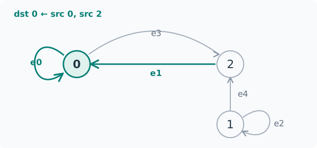
In storage order, the five edges are e0: 0 → 0, e1: 2 → 0, e2: 1 → 1,
e3: 0 → 2 and e4: 1 → 2. The self-loops
0 → 0 and 1 → 1 include the node itself as a message source.
Reverse edges are not added automatically: 1 → 2 does not imply 2 → 1.
The same graph as two arrays
CSR
is an array encoding of these arrows, not another graph computation. Tiga groups
incoming edges by destination: node 0 has sources [0, 2], node 1 has [1],
and node 2 has [0, 1]. Concatenating those lists gives col_idx = [0, 2, 1, 0, 1].
row_ptr = [0, 2, 3, 5] stores the group boundaries: array positions, not node IDs.
Destination 0 reads positions 0 up to but excluding 2; destination 1 reads 2 up
to 3; destination 2 reads 3 up to 5.
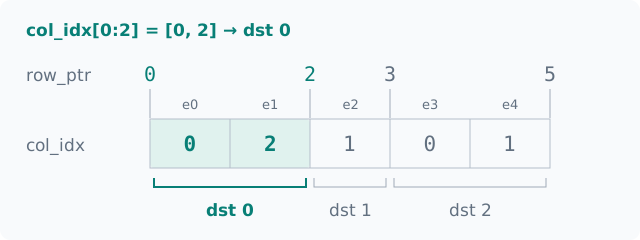
An ordinary Torch slice exposes the neighbors of a destination, without any IR:
row_ptr = torch.tensor([0, 2, 3, 5], dtype=torch.int64)
col_idx = torch.tensor([0, 2, 1, 0, 1], dtype=torch.int64)
dst_id = 0
begin, end = row_ptr[dst_id].item(), row_ptr[dst_id + 1].item()
sources = col_idx[begin:end].tolist()  # [0, 2]: sources sending to destination 0
graph = tg.Graph.from_csr(row_ptr, col_idx, num_src=3)
num_src=3 gives the number of source nodes. The destination count is
len(row_ptr) - 1, also 3 here; the edge count is len(col_idx), or 5.
Equal adjacent boundaries mean a destination has no incoming edges.
Graph determines only the first three columns below. The final column also
needs fields T, c and the calculation defined in edge().
| Destination | Edge interval | Source nodes | Weighted messages |
|---|---|---|---|
| 0 | [0, 2) |
[0, 2] |
2 * 1 + 3 * 3 = 11 |
| 1 | [2, 3) |
[1] |
4 * 2 = 8 |
| 2 | [3, 5) |
[0, 1] |
5 * 1 + 6 * 2 = 17 |
Other relation constructors exist, but construction and execution coverage are separate: see the support matrix.
2. Fields attach data to the graph
| Call binding | Meaning | Length in this example |
|---|---|---|
src={"T": T} |
Temperature per source node | 3 |
dst={"b": b} |
Bias per destination node | 3 |
edge={"c": c} |
Conductivity per edge, in CSR edge order | 5 |
src and dst are endpoint roles, not necessarily different node sets.
Even when both roles refer to the same nodes, they can carry different fields.
Field names belong to the program; T, b and c are not compiler keywords.
3. MessagePassing defines edge computation
Inside edge(), src.T is the current edge's source temperature and
edge.c is that edge's conductivity. One vectorized call covers the relation;
no Python loop over neighbors is needed.
The optional node() updates nodes after aggregation. Here it adds bias,
producing approximately [11.1, 8.2, 17.3].
Exact parameter rules, field shapes, the ndata shorthand and allowed
expressions are in the MessagePassing contract.
4. A reducer combines messages
A reducer
combines the incoming messages for one destination into a result.
tg.sum() sums, tg.mean() averages, and tg.prod() multiplies.
Start with a built-in; a custom algebra is not required.
Empty-row behavior and execution coverage differ between reducers; see the reducer guide.
Calls, results and gradients
The call returns a torch.Tensor. torch.autograd.grad obtains gradients
through the same definition without a handwritten backward function.
Node 0 affects the result through coefficients 2 and 5, so its temperature
gradient is 7.
Execution and troubleshooting explains policies, reference evaluation and caches. Torch-path planning diagnostics live on the kernel, not on Torch result objects.
Next
- MessagePassing contract: fields, parameters and call rules.
- Examples: select a workload.
- Compiler introduction: optional implementation reading.