Examples
This section provides practical examples for using torch-sla.
Quick Navigation
- Visualization:
spy()for sparsity pattern analysis - I/O Operations: Matrix Market & SafeTensors format support
- Linear Solve: Direct & iterative solvers with gradients
- Matrix Decompositions: SVD, Eigenvalue, LU factorization
- Advanced: Nonlinear solve, distributed computing
Visualization
Spy Plot (Sparsity Pattern)
Visualize the sparsity pattern of a sparse matrix using the .spy() method.
Code:
import torch
from torch_sla import SparseTensor

# Create a 2D Poisson matrix (5-point stencil)
n = 50
val, row, col = [], [], []
for i in range(n):
    for j in range(n):
        idx = i * n + j
        val.append(4.0); row.append(idx); col.append(idx)
        if j > 0: val.append(-1.0); row.append(idx); col.append(idx-1)
        if j < n-1: val.append(-1.0); row.append(idx); col.append(idx+1)
        if i > 0: val.append(-1.0); row.append(idx); col.append(idx-n)
        if i < n-1: val.append(-1.0); row.append(idx); col.append(idx+n)

A = SparseTensor(torch.tensor(val), torch.tensor(row), torch.tensor(col), (n*n, n*n))

# Visualize sparsity pattern
A.spy(title="2D Poisson (5-point stencil)")
Output Examples:
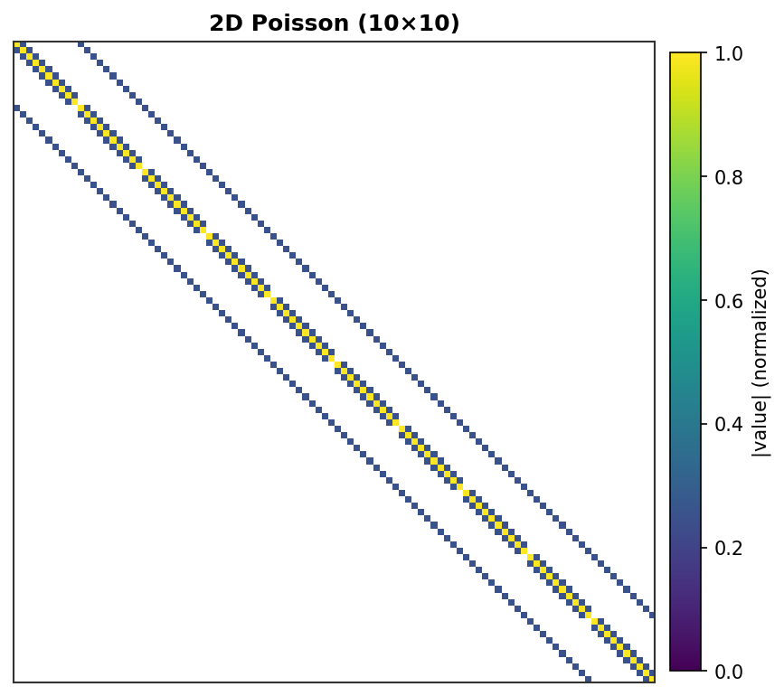
2D Poisson (10×10) - 100 DOF, 5-point stencil with grid lines¶ |
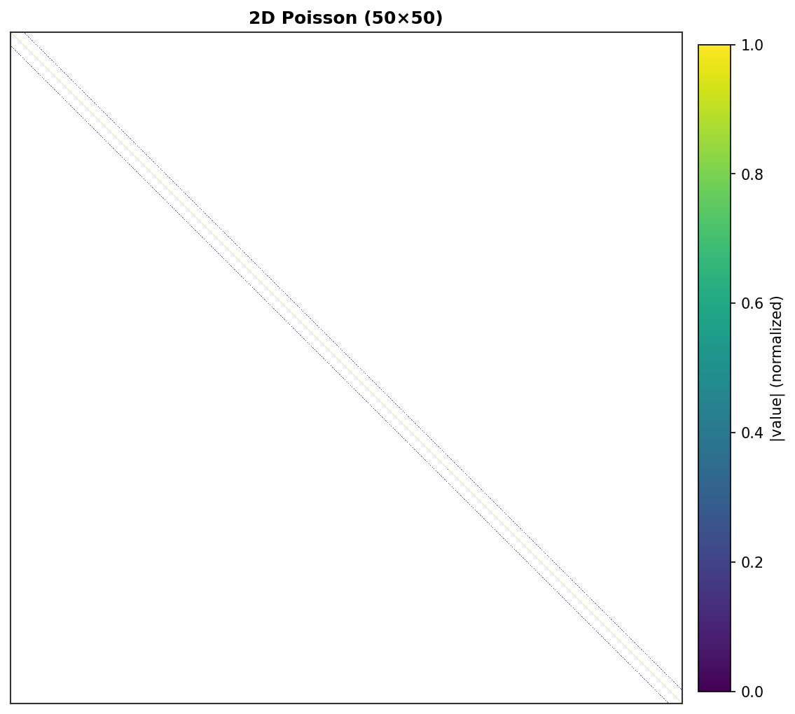
2D Poisson (50×50) - 2,500 DOF, band structure visible¶ |
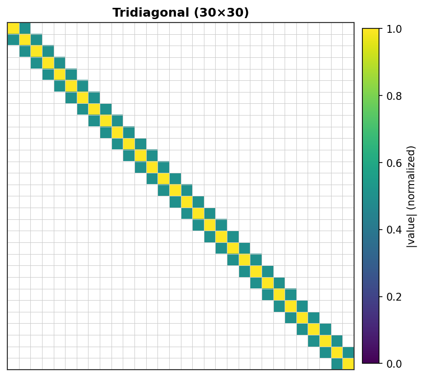
Tridiagonal (30×30) - Classic 1D Poisson pattern¶ |
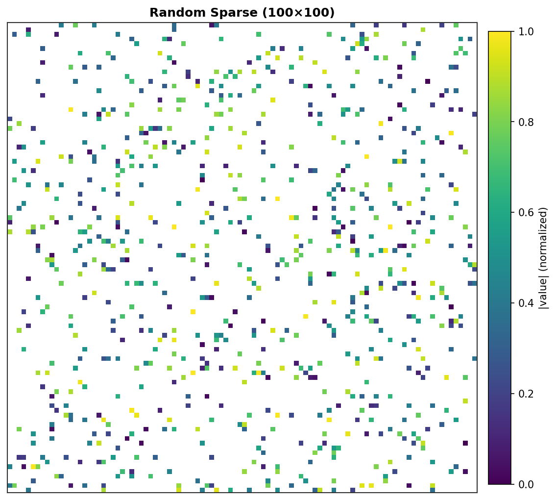
Random Sparse (100×100) - 800 random non-zeros¶ |
Each non-zero element is rendered as a colored pixel with intensity proportional to its absolute value. Zero elements are white.
I/O Operations
Matrix Market Format
Save and load sparse matrices in the standard Matrix Market (.mtx) format.
Code:
from torch_sla import SparseTensor, save_matrix_market, load_matrix_market

# Create a sparse matrix
A = SparseTensor(val, row, col, (100, 100))

# Save to Matrix Market format
save_matrix_market(A, "matrix.mtx", comment="My sparse matrix")

# Load from Matrix Market format
B = load_matrix_market("matrix.mtx", device="cuda")

# Verify
assert torch.allclose(A.to_dense(), B.to_dense())
File format (.mtx):
%%MatrixMarket matrix coordinate real general
% My sparse matrix
100 100 500
1 1 4.0
1 2 -1.0
...
SafeTensors Format
Save and load using the efficient safetensors format.
Code:
from torch_sla import SparseTensor

A = SparseTensor(val, row, col, shape)

# Save
A.save("matrix.safetensors")

# Load
B = SparseTensor.load("matrix.safetensors", device="cuda")

# Save distributed (for multi-GPU)
A.save_distributed("matrix_dist/", num_partitions=4)
Basic Usage
Basic Sparse Linear Solve
Solve a sparse linear system \(Ax = b\) using SparseTensor.
Linear System:
Given a sparse matrix \(A \in \mathbb{R}^{n \times n}\) and right-hand side \(b \in \mathbb{R}^n\), find \(x \in \mathbb{R}^n\) such that:
Solver Methods:
Direct solvers (LU, Cholesky): Exact solution, \(O(n^{1.5})\) for sparse
Iterative solvers (CG, BiCGStab): Approximate solution, \(O(k \cdot \text{nnz})\) where \(k\) is iterations
Problem:
This is a 3×3 symmetric positive definite (SPD) tridiagonal matrix from 1D Poisson discretization.
COO Format:
Index |
Row |
Col |
Value |
|---|---|---|---|
0 |
0 |
0 |
4.0 |
1 |
0 |
1 |
-1.0 |
2 |
1 |
0 |
-1.0 |
3 |
1 |
1 |
4.0 |
4 |
1 |
2 |
-1.0 |
5 |
2 |
1 |
-1.0 |
6 |
2 |
2 |
4.0 |
Solution:
Code:
import torch
from torch_sla import SparseTensor

# Create sparse matrix from dense (easier to read for small matrices)
dense = torch.tensor([[4.0, -1.0,  0.0],
                      [-1.0, 4.0, -1.0],
                      [ 0.0, -1.0, 4.0]], dtype=torch.float64)

A = SparseTensor.from_dense(dense)
b = torch.tensor([1.0, 2.0, 3.0], dtype=torch.float64)

x = A.solve(b)
Property Detection
Detect matrix properties for optimal solver selection.
Symmetry: \(A = A^T\)
Positive Definiteness: All eigenvalues \(\lambda_i > 0\)
For the tridiagonal matrix: \(\lambda_1 \approx 2.59, \lambda_2 = 4.0, \lambda_3 \approx 5.41\) (all positive → SPD)
Code:
from torch_sla import SparseTensor

# Using the tridiagonal matrix from above
dense = torch.tensor([[4.0, -1.0,  0.0],
                      [-1.0, 4.0, -1.0],
                      [ 0.0, -1.0, 4.0]], dtype=torch.float64)
A = SparseTensor.from_dense(dense)

is_sym = A.is_symmetric()              # tensor(True)
is_pd = A.is_positive_definite()       # tensor(True)
Gradient Computation
Compute gradients through sparse solve using implicit differentiation.
Implicit Differentiation:
Given \(x = A^{-1} b\), for a loss function \(L(x)\), we want \(\frac{\partial L}{\partial A}\) and \(\frac{\partial L}{\partial b}\).
From \(Ax = b\), differentiate both sides:
Solving for \(dx\):
Adjoint Method:
Define adjoint variable \(\lambda = A^{-T} \frac{\partial L}{\partial x}\), then:
Gradient formulas (summary):
Code:
import torch
from torch_sla import spsolve

val = torch.tensor([4.0, -1.0, -1.0, 4.0, -1.0, -1.0, 4.0],
                   dtype=torch.float64, requires_grad=True)
row = torch.tensor([0, 0, 1, 1, 1, 2, 2])
col = torch.tensor([0, 1, 0, 1, 2, 1, 2])
b = torch.tensor([1.0, 2.0, 3.0], dtype=torch.float64, requires_grad=True)

x = spsolve(val, row, col, (3, 3), b)
loss = x.sum()
loss.backward()

# val.grad, b.grad now contain gradients
Specify Backend and Method
Choose solver backend and method explicitly.
Available Options:
Backend |
Device |
Methods |
|---|---|---|
|
CPU |
|
|
CPU |
|
|
CUDA |
|
|
CUDA |
|
Code:
from torch_sla import SparseTensor

A = SparseTensor(val, row, col, (n, n))
b = torch.randn(n, dtype=torch.float64)

x1 = A.solve(b, backend='scipy', method='superlu')    # Direct
x2 = A.solve(b, backend='scipy', method='cg')         # Iterative (SPD)
x3 = A.solve(b, backend='scipy', method='bicgstab')   # Iterative (general)
Matrix Operations
Compute norms, determinants, and eigenvalues.
Frobenius Norm:
Determinant:
For the tridiagonal matrix: \(\det(A) = 56\)
Gradient Formula:
Code:
from torch_sla import SparseTensor

# Using the tridiagonal matrix from above
dense = torch.tensor([[4.0, -1.0,  0.0],
                      [-1.0, 4.0, -1.0],
                      [ 0.0, -1.0, 4.0]], dtype=torch.float64)
A = SparseTensor.from_dense(dense)

norm = A.norm('fro')                              # ≈ 7.21
det = A.det()                                     # 56.0 (with gradient support)
eigenvalues, eigenvectors = A.eigsh(k=2, which='LM')  # Top-2 eigenvalues
Batched Solve
Batched SparseTensor
Solve multiple systems with same sparsity pattern but different values.
Problem: Solve 4 systems with scaled matrices
Code:
import torch
from torch_sla import SparseTensor

val = torch.tensor([4.0, -1.0, -1.0, 4.0, -1.0, -1.0, 4.0], dtype=torch.float64)
row = torch.tensor([0, 0, 1, 1, 1, 2, 2])
col = torch.tensor([0, 1, 0, 1, 2, 1, 2])

batch_size = 4
val_batch = val.unsqueeze(0).expand(batch_size, -1).clone()
for i in range(batch_size):
    val_batch[i] = val * (1.0 + 0.1 * i)

A = SparseTensor(val_batch, row, col, (batch_size, 3, 3))
b = torch.randn(batch_size, 3, dtype=torch.float64)

x = A.solve(b)  # x.shape: [4, 3]
Multi-Dimensional Batch
Handle shapes like [B1, B2, M, N].
Example: 2 materials × 3 temperatures = 6 systems
Code:
import torch
from torch_sla import SparseTensor

B1, B2, n = 2, 3, 8
val_batch = val.unsqueeze(0).unsqueeze(0).expand(B1, B2, -1).clone()

A = SparseTensor(val_batch, row, col, (B1, B2, n, n))
b = torch.randn(B1, B2, n, dtype=torch.float64)

x = A.solve(b)  # x.shape: [2, 3, 8]
solve_batch for Repeated Solves
Efficient batch solve with same structure but different values.
Use Case: Time-stepping with fixed sparsity pattern
LU Decomposition: \(A = LU\), then solve \(Ly = b\), \(Ux = y\)
Code:
from torch_sla import SparseTensor

A = SparseTensor(val, row, col, shape)

val_batch = torch.stack([val * (1.0 + 0.01 * t) for t in range(100)])  # [100, nnz]
b_batch = torch.randn(100, n, dtype=torch.float64)

x_batch = A.solve_batch(val_batch, b_batch)  # [100, n]
SparseTensorList
Handle matrices with different sparsity patterns.
Use Case: FEM meshes with different element counts
Code:
from torch_sla import SparseTensor, SparseTensorList

A1 = SparseTensor(val1, row1, col1, (5, 5))
A2 = SparseTensor(val2, row2, col2, (10, 10))
A3 = SparseTensor(val3, row3, col3, (15, 15))

matrices = SparseTensorList([A1, A2, A3])

b_list = [torch.randn(5), torch.randn(10), torch.randn(15)]
x_list = matrices.solve(b_list)
Distributed Solve
Basic DSparseTensor
Create distributed sparse tensor with domain decomposition.
Domain Decomposition: Split 16-node grid into 2 domains
Each domain has owned nodes and halo/ghost nodes from neighbors.
Code:
from torch_sla import DSparseTensor

D = DSparseTensor(val, row, col, (16, 16), num_partitions=2)

for i in range(D.num_partitions):
    p = D[i]
    # p.num_owned, p.num_halo, p.num_local
2D Poisson Example
Create 2D Poisson matrix with 5-point stencil.
Stencil:
Code:
import torch
from torch_sla import DSparseTensor

def create_2d_poisson(nx, ny):
    N = nx * ny
    rows, cols, vals = [], [], []
    for i in range(ny):
        for j in range(nx):
            idx = i * nx + j
            rows.append(idx); cols.append(idx); vals.append(4.0)
            if j > 0:
                rows.append(idx); cols.append(idx - 1); vals.append(-1.0)
            if j < nx - 1:
                rows.append(idx); cols.append(idx + 1); vals.append(-1.0)
            if i > 0:
                rows.append(idx); cols.append(idx - nx); vals.append(-1.0)
            if i < ny - 1:
                rows.append(idx); cols.append(idx + nx); vals.append(-1.0)
    return (torch.tensor(vals), torch.tensor(rows), torch.tensor(cols), (N, N))

val, row, col, shape = create_2d_poisson(4, 4)
D = DSparseTensor(val, row, col, shape, num_partitions=2)
Scatter and Gather
Distribute global vectors to partitions and gather back.
Diagram:
Global:  [x0, x1, x2, x3, x4, x5, x6, x7]
                  ↓ scatter
Local:   [x0, x1, x2, x3, x6]  (P0 + halo)
         [x4, x5, x6, x7, x3]  (P1 + halo)
                  ↓ gather
Global:  [x0, x1, x2, x3, x4, x5, x6, x7]
Code:
from torch_sla import DSparseTensor

D = DSparseTensor(val, row, col, shape, num_partitions=2)
x_global = torch.arange(16, dtype=torch.float64)

x_local = D.scatter_local(x_global)
x_gathered = D.gather_global(x_local)
Halo Exchange
Exchange ghost node values between neighboring partitions.
References:
1D Decomposition Diagram:
Partition 0: Owned [0,1,2,3], Halo [4] ← from P1
Partition 1: Owned [4,5,6,7], Halo [3] ← from P0
Exchange Process:
Before: P0=[x0,x1,x2,x3,?], P1=[x4,x5,x6,x7,?]
                     ↓ halo_exchange_local()
After:  P0=[x0,x1,x2,x3,x4], P1=[x4,x5,x6,x7,x3]
Why needed: For \(y_3 = \sum_j A_{3,j} x_j\), node 3 needs \(x_4\) from P1.
Code:
from torch_sla import DSparseTensor

D = DSparseTensor(val, row, col, shape, num_partitions=4)
x_list = [torch.randn(D[i].num_local) for i in range(D.num_partitions)]

D.halo_exchange_local(x_list)
Iterative Solvers
PyTorch CG Solver
For large-scale problems (> 100K DOF), iterative methods are much faster than direct solvers.
Conjugate Gradient (CG) Algorithm:
For symmetric positive definite (SPD) matrix \(A\), CG minimizes:
The minimum is achieved at \(x^* = A^{-1} b\).
CG Iteration:
Starting from \(x_0\), with residual \(r_0 = b - Ax_0\) and search direction \(p_0 = r_0\):
Convergence:
CG converges in at most \(n\) iterations (exact arithmetic). With condition number \(\kappa = \lambda_{\max}/\lambda_{\min}\):
Preconditioning:
Preconditioned CG (PCG) solves \(M^{-1} A x = M^{-1} b\) where \(M \approx A\):
Jacobi: \(M = \text{diag}(A)\) — simple, effective
Incomplete Cholesky: \(M = \tilde{L} \tilde{L}^T\) — better for ill-conditioned
Convergence Example:
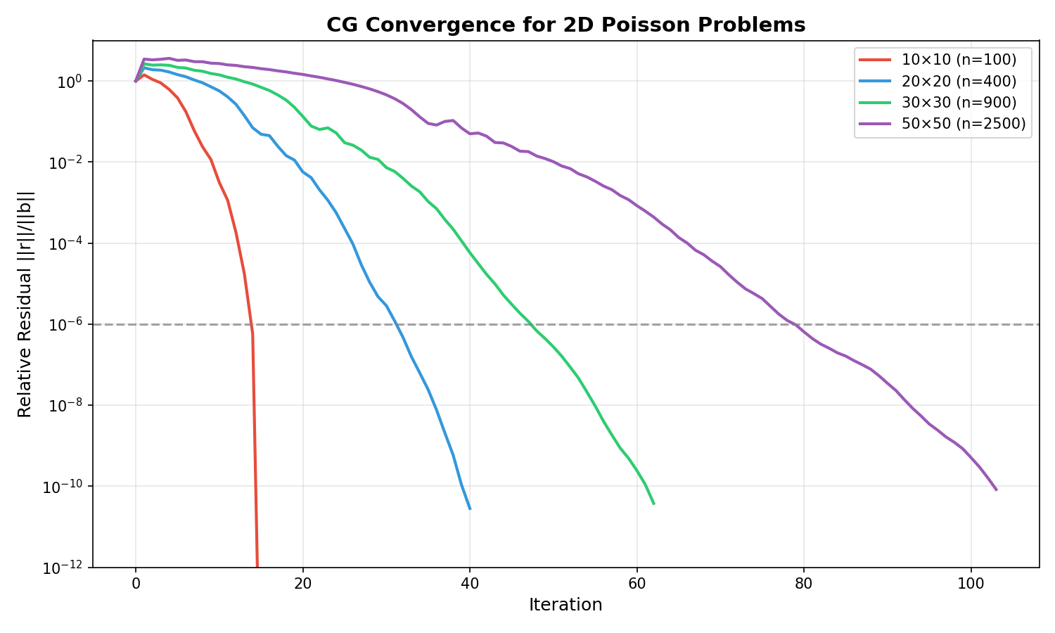
CG convergence for 2D Poisson problems of various sizes. Larger problems require more iterations due to worse conditioning.
Performance Comparison (1M DOF, NVIDIA H200):
Method |
Time |
Memory |
Best For |
|---|---|---|---|
|
0.5s ✅ |
~500 MB |
> 100K DOF, SPD |
|
7.8s |
~300 MB |
< 100K DOF, high precision |
Code:
from torch_sla import spsolve

# For large SPD systems, use PyTorch CG
x = spsolve(val, row, col, shape, b,
            backend='pytorch',
            method='cg',
            preconditioner='jacobi')
Preconditioners
Available preconditioners for iterative solvers:
Name |
Description |
Best For |
|---|---|---|
|
Diagonal scaling (default) |
General use, fastest |
|
Symmetric SOR (ω=1.5) |
Slow convergence problems |
|
Neumann series (degree=2) |
GPU-parallel |
|
Incomplete Cholesky |
Very ill-conditioned |
|
Algebraic Multigrid |
Float32, Poisson-like |
Recommendation:
Float64: Use
jacobi(simplest, fastest due to fewer iterations)Float32: Use
amg(reduces iterations, compensates for precision loss)
Code:
# Jacobi (default, recommended for float64)
x = spsolve(val, row, col, shape, b,
            backend='pytorch', preconditioner='jacobi')

# AMG (recommended for float32)
x = spsolve(val.float(), row, col, shape, b.float(),
            backend='pytorch', preconditioner='amg')
Mixed Precision
For memory-constrained scenarios, use mixed precision: - Matrix stored in Float32 (memory efficient) - Accumulation in Float64 (high precision)
Code:
x = spsolve(val_f32, row, col, shape, b_f32,
            backend='pytorch',
            method='cg',
            mixed_precision=True)  # Returns float64 solution
CUDA Usage
Move to CUDA
Transfer to GPU for CUDA-accelerated solving.
Performance: cuDSS/cuSOLVER can be 10-100× faster for large systems.
Code:
from torch_sla import SparseTensor

A = SparseTensor(val, row, col, shape)
A_cuda = A.cuda()

x = A_cuda.solve(b.cuda())
Backend Selection on CUDA
Auto Selection: cuDSS (preferred) → cuSOLVER (fallback)
Code:
x = A_cuda.solve(b_cuda, backend='cudss', method='lu')
x = A_cuda.solve(b_cuda, backend='cudss', method='cholesky')  # For SPD
x = A_cuda.solve(b_cuda, backend='cusolver', method='qr')
Advanced Examples
Nonlinear Solve with Adjoint Gradients
Solve nonlinear equations \(F(u, \theta) = 0\) with automatic differentiation using the adjoint method.
Problem Formulation:
Given a nonlinear residual function \(F: \mathbb{R}^n \times \mathbb{R}^p \to \mathbb{R}^n\), find \(u^*\) such that:
where \(\theta\) are parameters (e.g., forcing term, material properties).
Newton-Raphson Method:
Starting from initial guess \(u_0\), iterate:
where \(J_F = \frac{\partial F}{\partial u}\) is the Jacobian matrix.
Adjoint Method for Gradients:
For a loss function \(L(u^*)\), the gradient w.r.t. parameters is:
where the adjoint variable \(\lambda\) satisfies:
This is memory-efficient: O(1) instead of O(iterations) graph nodes.
Example: Nonlinear diffusion \(Au + u^2 = f\)
import torch
from torch_sla import SparseTensor

# Create stiffness matrix
A = SparseTensor(val, row, col, (n, n))

# Define nonlinear residual: F(u) = Au + u² - f
def residual(u, A, f):
    return A @ u + u**2 - f

# Parameters with gradients
f = torch.randn(n, requires_grad=True)
u0 = torch.zeros(n)

# Solve with Newton-Raphson
u = A.nonlinear_solve(residual, u0, f, method='newton')

# Gradients via adjoint method (memory efficient)
loss = u.sum()
loss.backward()
print(f.grad)  # ∂L/∂f
Methods:
Method |
Update Rule |
Convergence |
Best For |
|---|---|---|---|
|
\(u_{k+1} = u_k - J^{-1} F(u_k)\) |
Quadratic (fast) |
General nonlinear |
|
\(u_{k+1} = G(u_k)\) (fixed-point) |
Linear (slow) |
Mildly nonlinear |
|
Accelerated fixed-point with history |
Superlinear |
Memory-constrained |
Determinant with Gradient Support
Compute determinants of sparse matrices with automatic differentiation.
Determinant Definition:
For a square matrix \(A \in \mathbb{R}^{n \times n}\), the determinant is a scalar value that encodes important matrix properties:
Properties:
\(\det(AB) = \det(A) \det(B)\)
\(\det(A^T) = \det(A)\)
\(\det(A^{-1}) = 1/\det(A)\)
Matrix is singular ⟺ \(\det(A) = 0\)
Gradient Formula (Jacobi’s Formula):
For a differentiable loss \(L(\det(A))\):
This is computed efficiently using the adjoint method with \(O(1)\) graph nodes.
Implementation:
CPU: LU decomposition via SciPy SuperLU
CUDA: Dense conversion +
torch.linalg.detGradient: Adjoint method (solve \(A \mathbf{x} = \mathbf{e}_i\) for needed columns of \(A^{-1}\))
Example 1: Basic Determinant
import torch
from torch_sla import SparseTensor

# 3x3 tridiagonal matrix from dense
dense = torch.tensor([[4.0, -1.0,  0.0],
                      [-1.0, 4.0, -1.0],
                      [ 0.0, -1.0, 4.0]], dtype=torch.float64)

A = SparseTensor.from_dense(dense)
det = A.det()  # 56.0
Example 2: Gradient Computation
# Matrix with gradient tracking
dense = torch.tensor([[2.0, 1.0],
                      [1.0, 3.0]], dtype=torch.float64, requires_grad=True)

A = SparseTensor.from_dense(dense)
det = A.det()  # 5.0

# Compute gradient
det.backward()
print(dense.grad)  # [[3.0, -1.0], [-1.0, 2.0]]
Example 3: CUDA Support
# Move to CUDA
A_cuda = A.cuda()
det_cuda = A_cuda.det()  # Automatically uses CUDA backend
Example 4: Batched Determinants
# Multiple matrices with same structure
val_batch = torch.tensor([
    [2.0, 0.0, 0.0, 3.0],  # det = 6
    [1.0, 0.5, 0.5, 1.0],  # det = 0.75
], dtype=torch.float64)

A_batch = SparseTensor(val_batch, row, col, (2, 2, 2))
det_batch = A_batch.det()  # [6.0, 0.75]
Example 5: Optimization with Determinant Constraint
# Optimize matrix to achieve target determinant
val = torch.tensor([1.0, 0.5, 0.5, 1.0], requires_grad=True)
target_det = torch.tensor(2.0)
optimizer = torch.optim.Adam([val], lr=0.1)

for _ in range(50):
    optimizer.zero_grad()
    A = SparseTensor(val, row, col, (2, 2))
    loss = (A.det() - target_det) ** 2
    loss.backward()
    optimizer.step()
Example 6: Distributed Matrices
from torch_sla import DSparseTensor

# Create distributed sparse tensor
D = DSparseTensor(val, row, col, (n, n), num_partitions=4)

# Compute determinant (gathers all partitions)
det = D.det()  # Warning: requires data gather
Numerical Considerations:
Determinants can overflow/underflow for large matrices
For numerical stability, consider using log-determinant
Singular matrices (det ≈ 0) may cause LU decomposition to fail
Use
torch.float64for better numerical precision
Performance:
Matrix Size |
CPU (Sparse) |
CUDA (Dense) |
CPU-for-CUDA |
Notes |
|---|---|---|---|---|
10×10 |
0.3 ms |
1.0 ms |
0.5 ms |
CUDA 3x slower (dense overhead) |
100×100 |
0.3 ms |
0.3 ms |
0.5 ms |
Similar performance |
1000×1000 |
0.7 ms |
2.5 ms |
1.2 ms |
CUDA 3.6x slower (O(n³) vs O(n^1.5)) |
⚠️ Important Performance Note:
CUDA is slower than CPU for sparse determinants! This is because:
CPU uses sparse LU decomposition: O(nnz^1.5) time, O(nnz) memory
CUDA requires dense conversion: O(n³) time, O(n²) memory
cuSOLVER/cuDSS don’t expose sparse determinant computation
Recommendation: For CUDA tensors, use .cpu().det() instead of .det()
Eigenvalue Decomposition
Compute eigenvalues and eigenvectors of sparse matrices.
Eigenvalue Problem:
For a matrix \(A \in \mathbb{R}^{n \times n}\), find eigenvalues \(\lambda_i\) and eigenvectors \(v_i\) such that:
Symmetric Case (eigsh):
For symmetric matrices \(A = A^T\), eigenvalues are real and eigenvectors are orthonormal:
where \(\Lambda = \text{diag}(\lambda_1, \ldots, \lambda_n)\).
Algorithms:
ARPACK/LOBPCG: Iterative methods for sparse matrices, compute top-k eigenvalues
Shift-invert: For interior eigenvalues
Gradient Formula:
For a simple eigenvalue \(\lambda_i\) with eigenvector \(v_i\):
Code:
from torch_sla import SparseTensor

A = SparseTensor(val, row, col, (n, n))

# Largest eigenvalues (ARPACK/LOBPCG)
eigenvalues, eigenvectors = A.eigsh(k=6, which='LM')

# Smallest eigenvalues
eigenvalues, eigenvectors = A.eigsh(k=6, which='SM')

# For non-symmetric matrices
eigenvalues, eigenvectors = A.eigs(k=6)
Example Output:
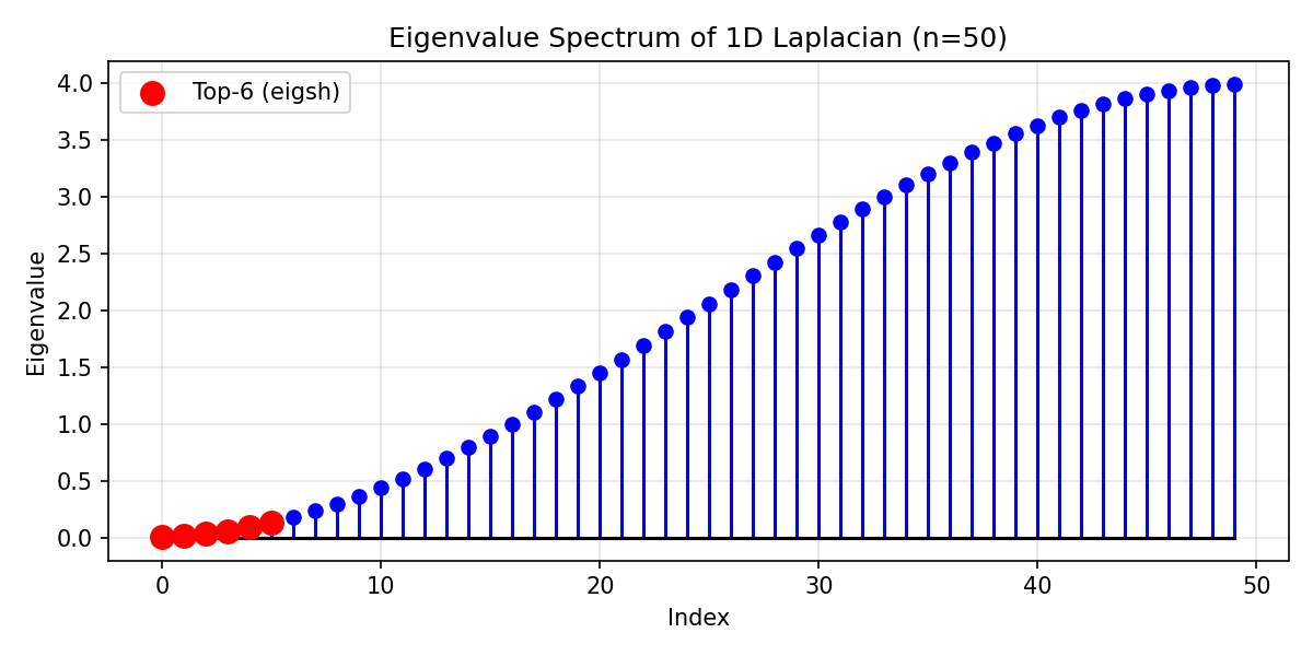
Eigenvalue spectrum of 1D Laplacian (n=50). Red points show the 6 smallest eigenvalues computed by eigsh().
Gradient support: Eigenvalue decomposition is differentiable!
val = val.requires_grad_(True)
A = SparseTensor(val, row, col, shape)
eigenvalues, _ = A.eigsh(k=3)
loss = eigenvalues.sum()
loss.backward()  # Gradients flow to val
SVD (Singular Value Decomposition)
Compute truncated SVD for sparse matrices.
SVD Definition:
For a matrix \(A \in \mathbb{R}^{m \times n}\), the SVD is:
where:
\(U \in \mathbb{R}^{m \times r}\): Left singular vectors (orthonormal columns)
\(\Sigma = \text{diag}(\sigma_1, \ldots, \sigma_r)\): Singular values (\(\sigma_1 \geq \sigma_2 \geq \ldots \geq 0\))
\(V \in \mathbb{R}^{n \times r}\): Right singular vectors (orthonormal columns)
Truncated SVD (rank-k approximation):
This is the best rank-k approximation in Frobenius norm (Eckart-Young theorem):
Relation to Eigenvalues:
\(\sigma_i^2\) are eigenvalues of \(A^T A\) (or \(A A^T\))
\(v_i\) are eigenvectors of \(A^T A\)
\(u_i\) are eigenvectors of \(A A^T\)
Applications:
Dimensionality reduction: PCA via SVD
Low-rank approximation: Matrix compression
Pseudoinverse: \(A^+ = V \Sigma^{-1} U^T\)
Example Output:
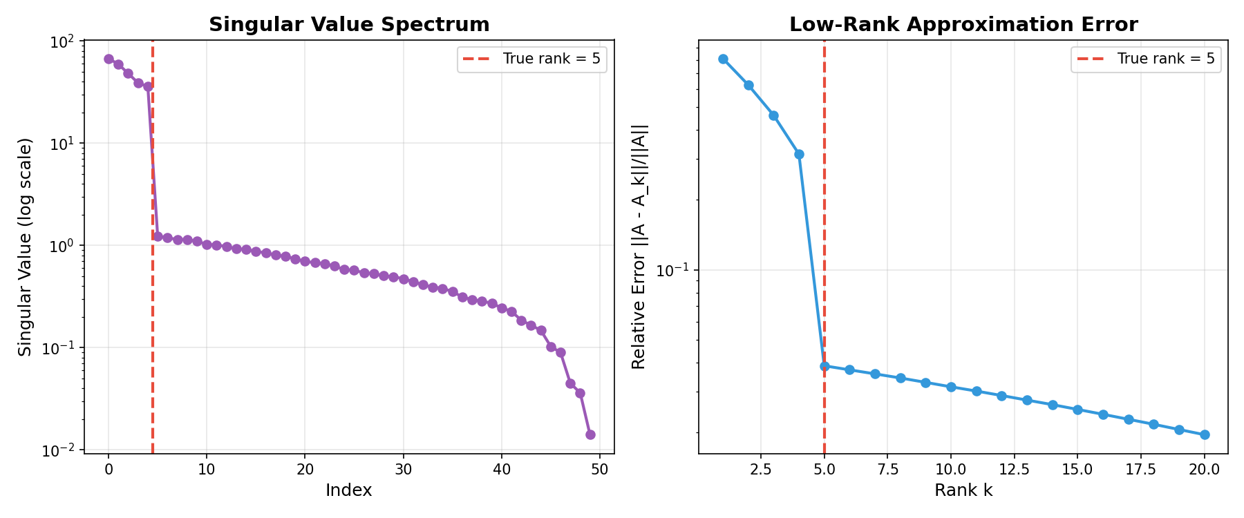
Left: Singular value spectrum showing rapid decay after true rank. Right: Approximation error decreases as rank increases.
Code:
from torch_sla import SparseTensor

A = SparseTensor(val, row, col, (m, n))

# Compute top-k singular values/vectors
U, S, Vt = A.svd(k=10)

# Low-rank approximation
A_approx = U @ torch.diag(S) @ Vt

# Relative approximation error
error = (A.to_dense() - A_approx).norm() / A.norm('fro')
LU Factorization for Repeated Solves
Cache LU factorization for efficient repeated solves with the same matrix.
LU Decomposition:
For a matrix \(A\), find lower triangular \(L\) and upper triangular \(U\) such that:
where \(P\) is a permutation matrix (for numerical stability).
Solving with LU:
To solve \(Ax = b\):
Factorize once: \(PA = LU\) — Cost: \(O(n^3)\) or \(O(\text{nnz}^{1.5})\) for sparse
Forward substitution: \(Ly = Pb\) — Cost: \(O(n^2)\) or \(O(\text{nnz})\) for sparse
Back substitution: \(Ux = y\) — Cost: \(O(n^2)\) or \(O(\text{nnz})\) for sparse
Complexity Savings:
For \(k\) solves with same matrix:
Without caching: \(O(k \cdot n^{1.5})\) (sparse direct)
With LU caching: \(O(n^{1.5} + k \cdot n)\) — up to \(\sqrt{n}\) faster!
Use Case: Time-stepping with fixed stiffness matrix
from torch_sla import SparseTensor

A = SparseTensor(val, row, col, shape)

# Factorize once (expensive)
lu = A.lu()

# Solve multiple RHS efficiently (cheap)
for t in range(100):
    b_t = compute_rhs(t)
    x_t = lu.solve(b_t)  # Fast solve using cached LU
Graph Neural Network Example
Use torch-sla for graph Laplacian operations in GNNs.
Code:
import torch
from torch_sla import SparseTensor

# Create adjacency matrix from edge list
edge_index = torch.tensor([[0, 1, 1, 2], [1, 0, 2, 1]])
edge_weight = torch.ones(4)

A = SparseTensor(edge_weight, edge_index[0], edge_index[1], (3, 3))

# Compute degree matrix
D = A.sum(dim=1)

# Normalized Laplacian: L = I - D^(-1/2) A D^(-1/2)
D_inv_sqrt = D.pow(-0.5)
A_norm = A * D_inv_sqrt.unsqueeze(1) * D_inv_sqrt.unsqueeze(0)
L = SparseTensor.eye(3) - A_norm

# Solve Laplacian system
x = L.solve(b)
Jupyter Notebook Examples
Interactive examples are available as Jupyter notebooks in the examples/ directory:
Notebook |
Description |
|---|---|
|
Basic solve, property detection, visualization |
|
Batched operations and SparseTensorList |
|
Determinant computation with gradient support (CPU & CUDA) |
|
Graph neural network with sparse Laplacian |
|
Nonlinear equations with adjoint gradients |
|
Spy plots and sparsity visualization |
|
Save/load with safetensors and Matrix Market |
|
Loading matrices from SuiteSparse Collection |
|
Distributed computing examples (matvec, solve, eigsh) |