Introduction¶

torch-sla (Torch Sparse Linear Algebra) is a memory-efficient library for sparse linear algebra in PyTorch. It provides differentiable sparse linear equation solvers with multiple backends, supporting both CPU and CUDA.

Key Features¶

Memory Efficient: Only stores non-zero elements — solve systems with millions of unknowns using minimal memory
Multiple Backends: Choose from SciPy, Eigen (C++), cuDSS, or PyTorch-native
Backend/Method Separation: Independently specify the backend and solver method
Auto-selection: Automatically choose the best backend and method based on device, dtype, and problem size
Gradient Support: Full gradient computation via PyTorch autograd with O(1) graph nodes
Batched Operations: Support for batched sparse tensors with shape [..., M, N, ...]
Property Detection: Automatic detection of symmetry and positive definiteness
Distributed Support: Distributed sparse matrices with halo exchange for parallel computing
Large Scale: Tested up to 169 million DOF with near-linear scaling

Recommended Backends¶

Based on extensive benchmarks on 2D Poisson equations (tested up to 169M DOF):

Recommended Backends¶
Problem Size	CPU	CUDA	Notes
Small (< 100K DOF)	`scipy+superlu`	`cudss+cholesky`	Direct solvers, machine precision
Medium (100K - 2M DOF)	`scipy+superlu`	`cudss+cholesky`	cuDSS is fastest on GPU
Large (2M - 169M DOF)	N/A	`pytorch+cg`	Iterative only, ~1e-6 precision
Very Large (> 169M DOF)	N/A	`DSparseMatrix` multi-GPU	Multi-GPU domain decomposition

Key Insights¶

PyTorch CG+Jacobi scales to 169M+ DOF with near-linear O(n^1.1) complexity
Direct solvers limited to ~2M DOF due to memory (O(n^1.5) fill-in)
Use float64 for best convergence with iterative solvers
Trade-off: Direct = machine precision (~1e-14), Iterative = ~1e-6 but 100x faster

Core Classes¶

SparseTensor¶

The main class for sparse matrix operations. Supports batched and block sparse tensors.

from torch_sla import SparseTensor

# Simple 2D matrix [M, N]
A = SparseTensor(values, row, col, (M, N))

# Batched matrices [B, M, N]
A = SparseTensor(values_batch, row, col, (B, M, N))

# Solve, norm, eigenvalues
x = A.solve(b)
norm = A.norm('fro')
eigenvalues, eigenvectors = A.eigsh(k=6)

SparseTensorList¶

A list of SparseTensors with different sparsity patterns.

from torch_sla import SparseTensorList

matrices = SparseTensorList([A1, A2, A3])
x_list = matrices.solve([b1, b2, b3])

DSparseTensor¶

Distributed sparse tensor with domain decomposition and halo exchange.

from torch_sla import DSparseTensor

D = DSparseTensor(val, row, col, shape, num_partitions=4)
x_list = D.solve_all(b_list)

LUFactorization¶

LU factorization for efficient repeated solves with same matrix.

lu = A.lu()
x = lu.solve(b)  # Fast solve using cached LU factorization

Backends¶

Available Backends¶
Backend	Device	Description	Recommended
`scipy`	CPU	SciPy backend using SuperLU or UMFPACK for direct solvers	CPU default
`eigen`	CPU	Eigen C++ backend for iterative solvers (CG, BiCGStab)	Alternative
`cudss`	CUDA	NVIDIA cuDSS for direct solvers (LU, Cholesky, LDLT)	CUDA direct
`cusolver`	CUDA	NVIDIA cuSOLVER for direct solvers	Not recommended
`pytorch`	CUDA	PyTorch-native iterative (CG, BiCGStab) with Jacobi preconditioning	Large problems (>2M DOF)

Methods¶

Direct Solvers¶

Direct Solver Methods¶
Method	Backends	Description	Precision
`superlu`	scipy	SuperLU LU factorization (default for scipy)	~1e-14
`cholesky`	cudss, cusolver	Cholesky factorization (for SPD matrices, fastest)	~1e-14
`ldlt`	cudss	LDLT factorization (for symmetric matrices)	~1e-14
`lu`	cudss, cusolver	LU factorization (general matrices)	~1e-14

Iterative Solvers¶

Iterative Solver Methods¶
Method	Backends	Description	Precision
`cg`	scipy, eigen, pytorch	Conjugate Gradient (for SPD) with Jacobi preconditioning	~1e-6
`bicgstab`	scipy, eigen, pytorch	BiCGStab (for general matrices) with Jacobi preconditioning	~1e-6
`gmres`	scipy	GMRES (for general matrices)	~1e-6

Quick Start¶

Basic Usage¶

import torch
from torch_sla import SparseTensor

# Create a sparse matrix from dense (easier to read for small matrices)
dense = torch.tensor([[4.0, -1.0,  0.0],
                      [-1.0, 4.0, -1.0],
                      [ 0.0, -1.0, 4.0]], dtype=torch.float64)

# Create SparseTensor
A = SparseTensor.from_dense(dense)

# Solve Ax = b (auto-selects scipy+superlu on CPU)
b = torch.tensor([1.0, 2.0, 3.0], dtype=torch.float64)
x = A.solve(b)

CUDA Usage¶

import torch
from torch_sla import SparseTensor

# Create on CPU, move to CUDA (using the matrix from above)
A_cuda = A.cuda()

# Solve on CUDA (auto-selects cudss+cholesky for small problems)
b_cuda = b.cuda()
x = A_cuda.solve(b_cuda)

# For very large problems (DOF > 2M), use iterative
x = A_cuda.solve(b_cuda, backend='pytorch', method='cg')

Nonlinear Solve¶

Solve nonlinear equations with adjoint-based gradients:

from torch_sla import SparseTensor

# Create stiffness matrix
A = SparseTensor(val, row, col, (n, n))

# Define nonlinear residual: A @ u + u² = f
def residual(u, A, f):
    return A @ u + u**2 - f

f = torch.randn(n, requires_grad=True)
u0 = torch.zeros(n)

# Solve with Newton-Raphson
u = A.nonlinear_solve(residual, u0, f, method='newton')

# Gradients flow via adjoint method
loss = u.sum()
loss.backward()
print(f.grad)  # ∂L/∂f

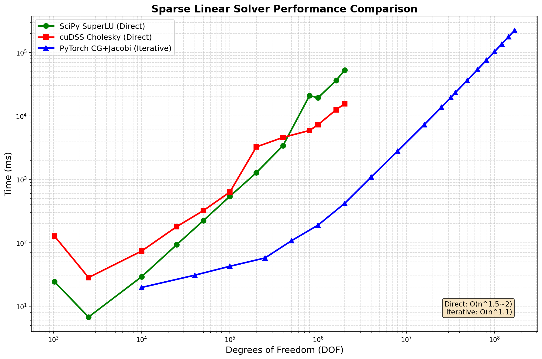
Benchmark Results¶

2D Poisson equation (5-point stencil), NVIDIA H200 (140GB), float64:

Performance Comparison¶

Performance (Time in ms)¶
DOF	SciPy SuperLU	cuDSS Cholesky	PyTorch CG+Jacobi	Notes	Winner
10K	24	128	20	All fast	PyTorch
100K	29	630	43		SciPy
1M	19,400	7,300	190		PyTorch 100x
2M	52,900	15,600	418		PyTorch 100x
16M	OOM	OOM	7,300		PyTorch only
81M	OOM	OOM	75,900		PyTorch only
169M	OOM	OOM	224,000		PyTorch only

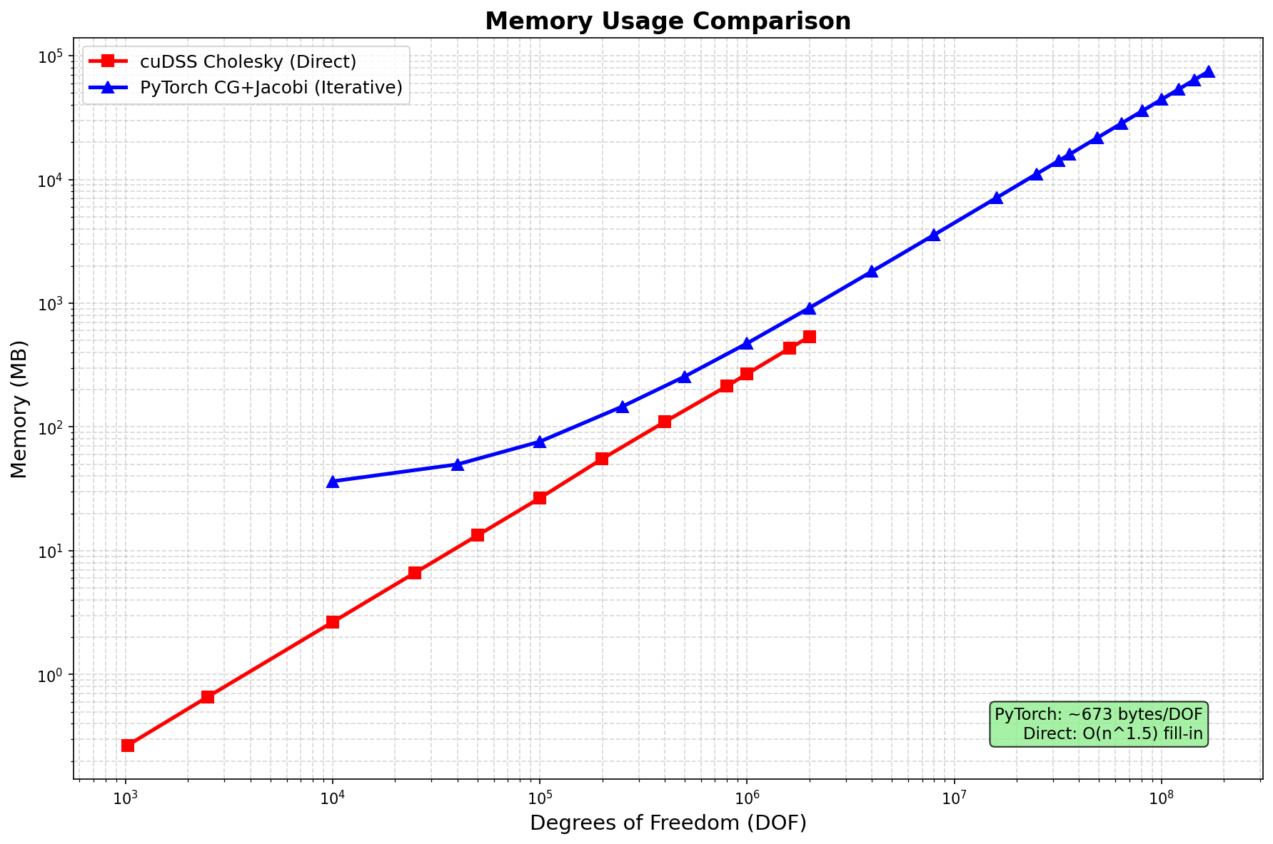
Memory Usage¶

Memory Characteristics¶
Method	Memory Scaling	Notes
SciPy SuperLU	O(n^1.5) fill-in	CPU only, limited to ~2M DOF
cuDSS Cholesky	O(n^1.5) fill-in	GPU, limited to ~2M DOF
PyTorch CG+Jacobi	O(n) ~443 bytes/DOF	Scales to 169M+ DOF

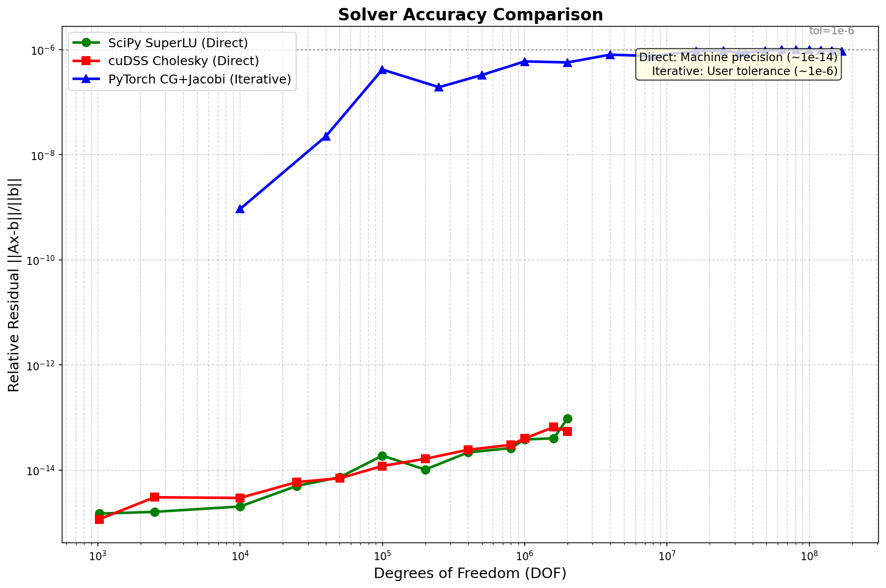
Accuracy¶

Accuracy Comparison¶
Method Type	Relative Residual	Notes
Direct (scipy, cudss)	~1e-14	Machine precision
Iterative (pytorch+cg)	~1e-6	User-configurable tolerance

Key Findings¶

Iterative solver scales to 169M DOF with O(n^1.1) time complexity
Direct solvers limited to ~2M DOF due to O(n^1.5) memory fill-in
PyTorch CG+Jacobi is 100x faster than direct solvers at 2M DOF
Memory efficient: 443 bytes/DOF (vs theoretical minimum 144 bytes/DOF)
Trade-off: Direct solvers achieve machine precision, iterative achieves ~1e-6

Distributed Solve (Multi-GPU)¶

3-4x NVIDIA H200 GPUs with NCCL backend, scales to 400M+ DOF:

CUDA (3-4 GPU, NCCL):

DOF	Time	Memory/GPU	GPUs
10K	0.1s	0.03 GB	4
100K	0.3s	0.05 GB	4
1M	0.9s	0.27 GB	4
10M	3.4s	2.35 GB	4
50M	15.2s	11.6 GB	4
100M	36.1s	23.3 GB	4
200M	119.8s	53.7 GB	3
300M	217.4s	80.5 GB	3
400M	330.9s	110.3 GB	3

Key Findings:

Scales to 400M DOF: Using 3x H200 GPUs (110 GB/GPU)
Near-linear scaling: 10M → 400M is 40x DOF, ~100x time
Memory efficient: ~275 bytes/DOF per GPU
CUDA 12x faster than CPU: 0.3s vs 7.4s for 100K DOF

# Run distributed solve with 3-4 GPUs
torchrun --standalone --nproc_per_node=3 examples/distributed/distributed_solve.py

Gradient Support¶

All operations support automatic differentiation via PyTorch autograd with O(1) graph nodes:

SparseTensor Gradient Support

Operation	CPU	CUDA	Notes
`solve()`	✓	✓	Adjoint method, O(1) graph nodes
`eigsh()` / `eigs()`	✓	✓	Adjoint method, O(1) graph nodes
`svd()`	✓	✓	Power iteration, differentiable
`nonlinear_solve()`	✓	✓	Adjoint, params only
`@` (A @ x, SpMV)	✓	✓	Standard autograd
`@` (A @ B, SpSpM)	✓	✓	Sparse gradients
`+`, `-`, `*`	✓	✓	Element-wise ops
`T()` (transpose)	✓	✓	View-like, gradients flow through
`norm()`, `sum()`, `mean()`	✓	✓	Standard autograd
`to_dense()`	✓	✓	Standard autograd

DSparseTensor Gradient Support

Operation	CPU	CUDA	Notes
`D @ x`	✓	✓	Distributed matvec with gradient
`solve_distributed()`	✓	✓	Distributed CG with gradient
`eigsh()` / `eigs()`	✓	✓	Distributed LOBPCG
`svd()`	✓	✓	Distributed power iteration
`nonlinear_solve()`	✓	✓	Distributed Newton-Krylov
`norm('fro')`	✓	✓	Distributed sum
`to_dense()`	✓	✓	Gathers data (with warning)

Key Features:

SparseTensor uses O(1) graph nodes via adjoint method for solve(), eigsh()
DSparseTensor uses true distributed algorithms (LOBPCG, CG, power iteration)
No data gather required for DSparseTensor core operations
For nonlinear_solve(), gradients flow to the parameters passed to residual_fn

Performance Tips¶

Use float64 for iterative solvers: Better convergence properties
Use cholesky for SPD matrices: 2x faster than LU
Use scipy+superlu for CPU: Best balance of speed and precision
Use cudss+cholesky for small CUDA problems: Fastest direct solver (< 2M DOF)
Use pytorch+cg for large problems: Memory efficient, scales to 169M+ DOF on single GPU
Use multi-GPU for very large problems: DSparseMatrix supports domain decomposition, 3 GPUs can reach 500M+ DOF
Avoid cuSOLVER: cudss is faster and supports float32
Use LU factorization for repeated solves: Cache with A.lu()

Citation¶

If you use torch-sla in your research, please cite our paper:

Paper: arXiv:2601.13994 - Differentiable Sparse Linear Algebra with Adjoint Solvers and Sparse Tensor Parallelism for PyTorch

@article{chi2026torchsla,
  title={torch-sla: Differentiable Sparse Linear Algebra with Adjoint Solvers and Sparse Tensor Parallelism for PyTorch},
  author={Chi, Mingyuan},
  journal={arXiv preprint arXiv:2601.13994},
  year={2026},
  url={https://arxiv.org/abs/2601.13994}
}