Computational Physics Question Card

1. RNG

1. What is Mersenne number? what is Mersenne prime number ?

   $M_n = 2^n-1$, when $M_n$ is prime

2. What is the advantage and disadvantage of multiplicative RNG and additive RNG?

   multiplicative simpler, faster, not good sequence

   additive complex, slower, better sequence

3. How many RNG algorithm do you remember?

   congruential, lagged fibonacci RNG

Congruential

1. What is Congruential RNG? Is it additive or Multiplicative?

   $x_i = (cx_{i-1})\text{mod}p$, multiplicative

2. What’s the max period or congruential RNG? When achieve it?

   $p-1$, when $p$ is a Mersenne prime number , $c^{p-1}mod~p = 1$

Lagged Fibonacci

1. What is Lagged Fibonacci RNG? Is it additive or Multiplicative?

   $x_{i+1} = (x_{i-c}+x_{i-d})\text{mod}2$, $c,d\in\{1,\cdots,i-1\},d\le c$ additive

2. How to generate the initial sequence before $c$

   use a congruential generator

3. What’s the max period?

   $2^c - 1$

4. What condition should the parameter $c,d$ satisfy? and the smallest number for it?

   $T_{c,d}(z) = 1+z^c + z^d $ (Zieler Trinomial)cannot be factorized, (250,103)

How good is RNG?

1. What kind of method could be used to measure RNG?

   square test, cube test, $\chi^2$ test, average value, spectral analysis, serial correlation test

2. What is square test?

   $(s_i,s_{i+1})\forall i$ , no cluster means good

3. What is cube test?

   $(s_i,s_{i+1},s_{i+1})\forall i$, should be distributed homogenously

4. What is $\chi^2$ test

   the distribution around the mean value should behave like a Gaussian distribution

5. What is average test?

   $\underset{N\to \infin}{lim}\frac{1}{N}\sum_{i=1}^N s_i = \frac{1}{2}\quad\forall s_i\in[0,1]$

6. What is spectral analysis?

   $\mathcal F(s)$ should correspond to a uniform distribution

Quasi Monte Carlo

1. What is quasi Monte Carlo approches?

   use low-discrepancy sequence for Monte Carlo sampling

2. What is the error bounds in quasi-Monte Carlo? is the error bounds deterministic?

   $\mathcal O(\frac{log(N)^d}{N})$ $d$ is the problem dimension, $N$ is number of sampling,yes

3. What is the error of Monte Carlo sampling? When quasi MC is better than MC?

   $\mathcal O(\frac{1}{\sqrt{N}})$, number of samples is large enough

4. What is the advantage of quasi MC?

   quasi MC better convergence as $N$ increase, and error bounds is deterministic

Discrepancy and low-discrepancy sequence

1. What is D-star discrepancy?

   $$D^*(x_1,\cdots,x_n) = \underset{0\le v_j\le 1,j=1,\cdots,d}{sup}\left|\frac{1}{N}\sum_{i=1}^N\prod_{j=1}^d 1_{0\le x_j^i\le v_j} - \prod_{j=1}^d v_j\right|$$

   for every subset $E$ of $[0,1]^d$ get the biggest difference between the volume and average points density.

2. How to judge if a sequence $x_1,\cdots,x_n\in[0,1]^d$ is a low discrepancy sequence?

   $$D^*(x_1,\cdots,x_n)\le c(d)\cdot\frac{log(N)^d}{N}$$

Non Uniform Distribution

1. What are two method to perform transformation?

   mapping, rejection method

2. How do mapping work for unit sphere from $X,Y\sim\text{Unif}(0,1)$?

   $$\begin{aligned} \int_0^X\int_0^Y 1dxdy &= \frac{1}{4\pi}\int_0^\Theta\int_0^\phi \text{sin}\phi d\phi d\theta \\ XY &= \frac{1}{4\pi}(1-\text{cos}\phi)\theta \\ \theta &= 2\pi X\\ \phi &= \text{arccos}(1-2Y) \end{aligned}$$

3. How do mapping work for exponential distribution?

   the exponential distribution is defined as $P(y) = ke^{-yk}$

   $$\begin{aligned} \int_0 ^ y ke^{-y'k}dy' &= \int_0^z P_u(z')dz' = z\\ z &= 1-e^{-yk}\\ y &= -\frac{1}{k}ln(1-z) \end{aligned}$$

4. How do mapping work for gaussian? (Box-Muller transform)

   the gaussian distribution is written as $P(y) = \frac{1}{\sqrt{\pi\sigma}}e^{-\frac{y^2}{\sigma}}$

   $$\begin{aligned} z_1z_2 &= \int_0^{y_1}\int_0^{y_2}\frac{1}{\pi \sigma}e^{-\frac{y_1'^2 + y_2'^2}{\sigma}}dy_1'dy_2' = \frac{1}{\pi\sigma}\int_0^\phi \int_0^r e^{-\frac{r'^2}{\sigma}}r'dr'd\phi' \\ &= \frac{\phi}{2\pi}(1-e^{-\frac{r^2}{\sigma}}) = \underset{z_1}{\underbrace{\frac{1}{2\pi}arctan(\frac{y_1}{y_2})}}\underset{z2}{\underbrace{(1-e^{-\frac{y_1^2+y_2^2}{\sigma}})}} \\ y_1 &= \sqrt{-\sigma ln(1-z_2)}sin(2\pi z_1)\\ y_2 &= \sqrt{-\sigma ln(1-z_2)}cos(2\pi z_1) \end{aligned}$$

5. What condition should transformation method satify?

   integrability, invertibility

6. How to make rejection faster?

   individual box(Riemann-integral)

Speedup

1. What is the Amdahl’s law?

   $T(p) = (\alpha + \frac{1-\alpha}{p})T(1)$ ,$\alpha$ is the sequential part, $p$ is the speed up ratio

2. How many methods do you know in Julia for parallel programming?

   asynchronous, multi-threading, distributed, gpu

2. Percolation

1. What is the main goal of percolation?

   study the formation of clusters

2. What are two types of percolation?

   site/bond percolation

3. What is percolated ?

   as occupation rate $p$ go to some point, cluster size will go to infinite (phase transition)

Phase Transition

1. What name is the phase transition occuring in percolation?

   second-order phase transition

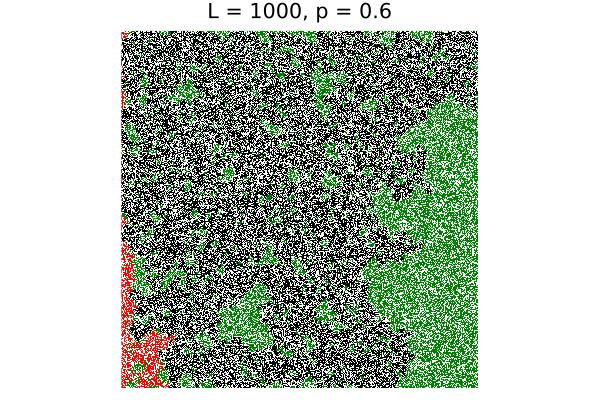
2. What is the percolation strength, and it’s definition near at $p=1 $ and $p<p_c$

   infinite cluster $P(p<p_c) = 0$, $P(p=1)=1$ , $P(p\gtrsim p_c)\sim|p-p_c|^\beta$ ,$\beta$ is percolation strength/order parameter, it strongly depends on the problem

3. which lattice has the highest 2d threshold $p_c$ site and $p_c$ bond ?

   honeycomb

4. what is wrapping probability?

   the probability system is percolated. $W(p)=0~if~p<p_c~else~1$

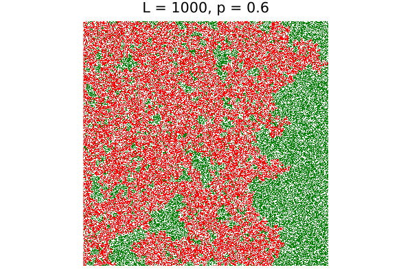
Cluster Size Distribution

1. What is cluster size distribution?

   $$n_s(p) = \underset{L\to\infin}{lim}\frac{N_s(p,L)}{L}$$

   $p$ : occupation probability

   $L$ : system’s side length

   $N_s(p,L)$ : number of clusters of size $s$

2. What phenomenon will you find for cluster size distribution with different $p$?

   

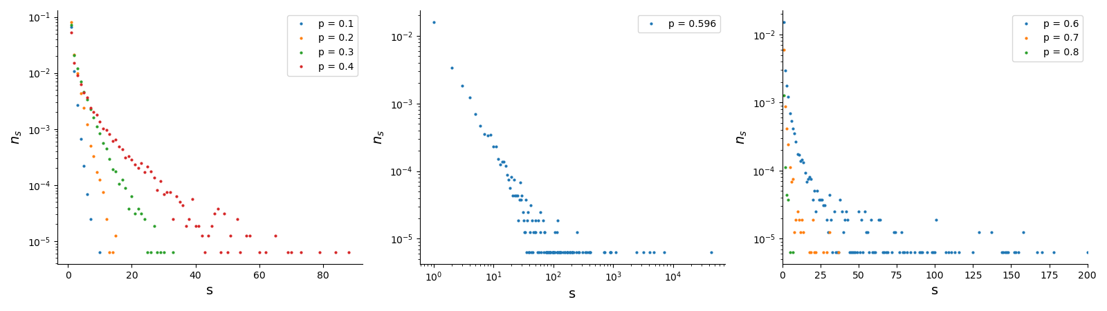
   $p<p_c$, as $p\uparrow$ , $s-ln(n_s)$ are higher

   $p=p_c$, straight line

   $p > p_c$, as $p\uparrow$, $s-ln(n_s)$ are lower

3. What do you observe in the $\chi^2$ test for the cluster size? ($\chi=\sum_s s^2\frac{N_s}{N_{clusters}}$)

   

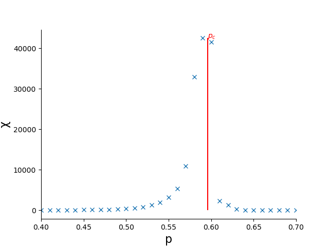
   There is a spike near $p_c$

Burning Method

1. What information can burning method provide?

   a boolean feedback(yes or no percolated),

   minimal path length

2. Write a short code for burning method

   

   def burning_method(L=16):
       lattice = np.random.randint(0, 2, (L, L)) # 0 empty 1 occupied
       t = 2
       lattice[0][lattice[0]==1] = t
       while True:
           cells = np.where(lattice == t)[0]
           burn_neighbor = False
           for cell in cells:
               for neighbor in neighbors[cell]:
                   if neighbor == 1:
                       lattice[neighbor] = t+1
                       burn_neighbor = True
           if not burn_neighbor
           	break            
           t += 1

3. How to count the largest cluster size of a random generated lattice?

   

   similar to the burning algorithm but from another side.

Hoshen-Kopelmann Algorithm

1. What is the Hoshen-Kopelman used for?

   

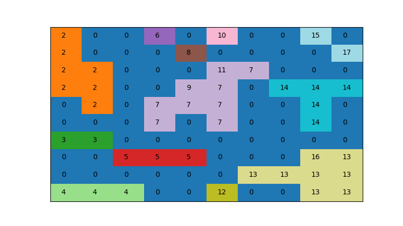
   know how the different clusters are distributed

2. What is the complexity of Hoshen-Kopelman Algorithm?

   linear to the number of sites

3. Write a short code for Hoshen-Kopelmann algorithm

   def hoshen_kopelmann(L=16):
       lattice = np.random.randint(0, 2, (L, L))
       M = np.array([0,0]) # cluster counter
       for i in range(L):
           for j in range(L):
               if lattice[i,j] == 1:
                   if no_left(i,j) and no_top(i,j): # no left and no top neighbor
                       lattice[i,j] = len(M);
                     	M = np.append(M, 1)
                   elif no_left(i,j) ^ no_top(i,j): # either left or top neighbor 
                       k0 = lattice[i-1,j] if no_left(i,j) else lattice[i, j-1]
                       lattice[i,j] = k0
                       M[k0] += 1
                   else: # has left and top neighbors
                       k1, k2 = lattice[i-1, j], lattice[i, j-1]
                      	lattice[i,j] = k1
                       M[k1] = M[k1] + M[k2] + 1
                       M[k2] = -k1

3. Fractal

1. what is the fractal dimension?

   $$\underset{\varepsilon\to 0}{lim}\frac{V_\varepsilon^*}{\varepsilon^d} = \left(\frac{L}{\varepsilon }\right)^{d_f} \quad d_f = \underset{\varepsilon\to 0}{lim}\frac{\text{log}(V^*/\varepsilon^d)}{\text{log}(L/\varepsilon)}$$

   for fractal dimension $a^{d_f}$, if the length is stretched by factor of $a$, it’s volume(mass) grows by $a^{d_f}$

2. What is the fractal dimension of Sierpinski triangle?

   $\frac{\text{log}(3)}{\text{log}(2)} \approx 1.585$

Sandbox method

1. Write a short code for sandbox method

   def sandbox(lattice):
       R_2s   = np.arange(1,lattice.shape[0] // 2) # half size of R
       NRs    = np.zeros_like(R_2s)
       Rs     = R_2s * 2 
       for i,R_2 in enumerate(R_2s): 
           NRs[i] = lattice[R_2:-R_2,R_2:-R_2].sum()
       plot_log_log(NRs, Rs)

   growing boxes from center

2. what is the slope of the log-log plot ($N(R)-R$) of sandbox method

   fractal dimension $d_f$

Box counting method

1. write a short code for box counting method

   def box_counting(lattice):
       epsilon = lattice.shape[0]
       N_epsilons = []
       epsilons   = []
       while epsilon >= 1:
           N_epsilon = maxpool2d(lattice, epsilon).sum()
           epsilon = epsilon // 2
       plot_log_log(N_epsilons,epsilons)

2. what is the slope of the log-log plot ($N(R)-R$) of box counting algorithm

   fractal dimension $d_f$

Fractals & Percolation

1. What is the correlation function $c(r)$ ? And what does the expression mean?

   $$c(r) = \frac{\Gamma(d/2)}{2\pi^{d/2}r^{d-1}\Delta r}[M(r+\Delta r)-M(r)]$$

   $c(r)$ counts the filled sites within a $d$ dimension hyper shell of thick $\Delta r$ with radius $r$ and normalize by the surface area

2. What is the common relation for $c(r)-r$

   $c(r)$ decrease exponentially with $r$ , $c(r)\propto C+exp\left(-\frac{r}{\xi}\right)$ , $\xi$ is correlation length, propotional to the radius of a typical cluster

3. When is correlation $\xi$ singular?

   $\xi$ is singular at $p_c$, $\xi\propto |p-p_c|^{-\nu}$ where $\nu=\begin{cases}4/3&d=2\\0.88&d=3\end{cases}$

4. How does $c(r)$ behave when $\xi$ is singular?

   $c(r)\propto r^{-(d-2+\eta)}$, where $\eta=\begin{cases}5/24&d=2\\-0.05&d=3\end{cases}$

5. What’s the relation between the fractal dimension $d^f$ and dimension $d$ ?

   $d^f = d - \frac{\beta}{\nu}$

4. Cellular Automata

1. Illustrate the components $\mathcal L,\psi, R,\mathcal N$ defining a cellular automata

   $\mathcal L$: lattice, $\psi(\textbf{r},t)$: state of each site $\textbf{r}$ at time $t$ , $R$ update rules, $\mathcal N$: neighbors

2. What is the synchronous dynamics?

   $R$ rules applied simultaneously to all sites

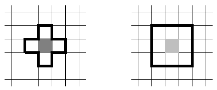
3. What’s the difference between Von Neumann neighborhood and Moore neighborhood?

   Von Neumann: 4, Moore: 8

   

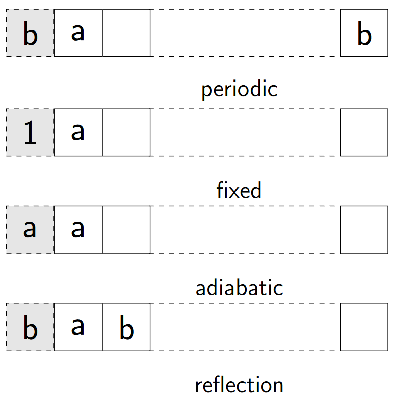
4. What’s the four types of boundaries?

   periodic, fixed, adiabatic, reflection

   

Game of Life

1. What is the neighborhood for Game of Life?

   Moore neighborhood

2. What’s the rule $R$ for Game of Life ?

   neighbors	action
   $n<2$	dead, because of isolation
   $n=2$	unchange
   $n=3$	birth
   $n>3$	dead, because of over population

3. List some periodic pattern in Game of Life

   pattern	animation
   glider
   glider gun

Langton Ant

1. What’s the observation of the Langton Ant?

   • chaotic phase of about 10000 steps
   • form highway
   • walk on highway

2. What’s the rule $R$ for Langton Ant?

   cell state	action
   white	turn $90\degree$ left, and paint the cell gray
   gray	turn $90\degree$ right, and paint the cell white

Traffic model

1. Consider one-dimension Cellular Automata with $\mathcal N$ as nearest neighbors. What does $c=101$ mean?

   $10_{10} = 01100101_{2}$ which stands for rule

   entries	111	110	101	100	011	010	001	000
   $\alpha$	0	1	1	0	0	1	0	1

2. In above setting, how many possible rules for 1 D Cellular Automata with $q=3$?

   $2^8=256$

3. What phenomenon will you observe for number of moving cars when $c=184$

   

   

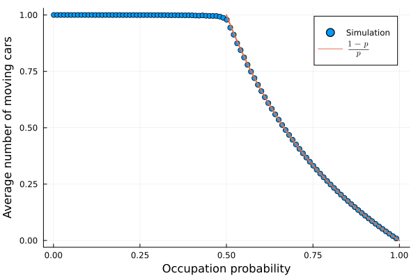
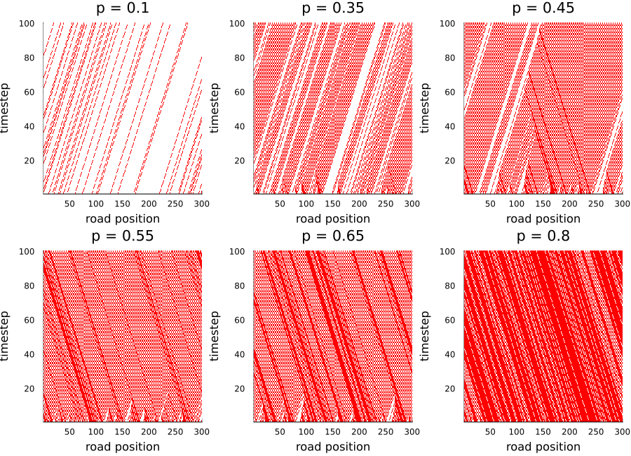
   when $p>0.5$, traffic jam will happen

​

HPP model

1. What does the HPP lattice look like?

   HPP lattice is defined on a 2d square lattice, also one could use hexagonal grid with two possible result

2. Describe the steps of HPP model.

   

   • collision
   • propagation/streaming

   

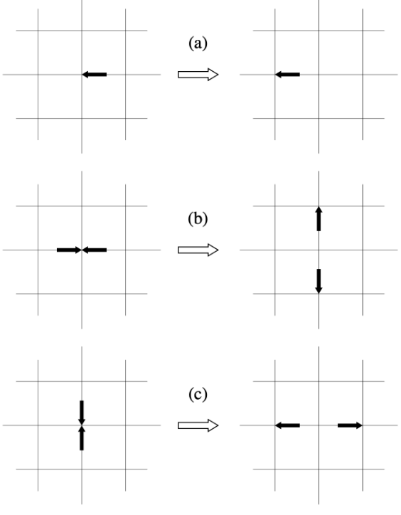
3. How many bits of information at each site are enough for HPP model ?

   4, $\psi(r,t)=(1011)$: three particles entering the site in direction 1,3,4

5. Monte Carlo

1. the main steps of a MC method?

   • random choose a new configuration in phase space,

   • accept or reject new configuration,

   • compute physical quantity and add it to the averaging procedure,

   • repeat

2. with is the error $\Delta$ of MC? is it depend on the dimension?

   $\Delta \propto \frac{1}{\sqrt{N}}$, no

Buffon’s Needle

1. Suppose the length of the needle is $l$ and distance of grid is $t$. What is the probability of the needle cross the line?

   $2l / (πt)$

Integration

1. when simple sampling MC integration works well?

   when $g(x)$ is smooth

2. what’s the error of conventional integration(Trapezoidal Rule) ?

   $\Delta \propto N^{-\frac{2}{d}}$

3. What’s the error in simple MC integration?

   $\Delta \propto \frac{1}{\sqrt N}$, it’s independent of the dimension $d$

4. What’s the curcial points for MC method(MC more efficient than conventional method)?

   $d_{crit} = 4$

5. Describe the steps for high dimension integration using MC.

   • choose particle position
   • make sure new sphere not overlap with pre-existing spheres. If it overlap, reject and sample again

6. Given a distribution $g(x)$ better enclose the $f(x)$, describe the steps for sampling better $x$

   • $u\sim P_u(0,1)$
   • $x=G^{-1}(u), G(x)=\int g(x)dx$
   • $y = P_u(0,g(x))$
   • if y > $f(x)$ try again, else return $x$

Importance Sampling

1. Given the $x$ sampling from $g(x)$ which is better enclose $f(x)$, how to integrate $f(x)$ using Importance Sampling?

   $$I\sim \frac{1}{N}\sum_{i=1}^N\frac{f(x_i^G)}{g(x_i^G)}$$

Control Variate

1. What is Control Variate?

   $$I = \int_a^b f(x)dx = \int_a^b(f(x)-g(x))dx +\int_a^b g(x)dx$$

2. If I want to use control variates, what condition should $g(x)$ satisfy

   • $\text{Var}(f-g)<\text{Var}(f)\Rightarrow 2\text{Cov}(f,g)>\text{Var}(g)$
   • $\int_a^b g(x)dx$ is known

Quasi Monte Carlo

1. What is Quasi Monte Carlo?

   use low discrepancy generator to choose $x$

2. What’s the theoretical error bound for Quasi Monte Carlo?

   $$\mathcal O\left(\frac{(\text{log} N)^d}{N}\right)$$

3. Does the convergence for Quasi Monte Carlo faster than theoretical?

   yes

4. When does Quasi Monte Carlo better than the Monte Carlo?

   $N>2^d$

Multi Level Monte Carlo

1. For a $L$ level MLMC, the cost/variance/ for each level is $C_l,V_l$, what’s the cost/variance/sample number for MLMC?

   $$\mathbb E[P_L ] = \mathbb E[P_0] + \sum_{l=1}^L \mathbb E [P_l - P_{l-1}]$$

   $$N_l = \mu \sqrt{\frac{V_l}{C_l}}\quad C = \sum_{l=1}^L C_l N_l \quad \text{Var} = \sum_{l=1}^L V_l N^{-1}_l$$

6. Markov Chain

1. given the transition probability $T$ and acceptance probability $A$, what’s the overall probability of a configuration?

   $$W(X\to Y) = T(X\to Y)\cdot A(X\to Y)$$

2. What’s the master equation for the evolution of the probability ?$p(X,\tau)$

   $$\frac{p(X,\tau)}{d\tau}=\sum_{Y\neq X}p(Y)W(Y\to X)-\sum_{Y\neq X}p(X)W(X\to Y)$$

3. What’s the three condition a Markov Chain should satisfy?

   • Ergodicitty: $\forall X,Y\quad W(X\to Y)>0$
   • Normalization: $\sum_Y W(X\to Y)=1$
   • Homogeneity: $\sum_Y p(Y)W(Y\to W)=p(X)$

4. What’s Detailed Balance ?

   $\frac{dp(X,\tau)}{d\tau}=0$ steady state of the Markov process

M(RT)$^2$ Algorithm

1. What’s Metropolis algorithm?

   $$A(X\to Y) = \text{min}\left(1,\frac{p_{eq}(Y)}{p_{eq}(X)}\right)$$

2. What’s M(RT)$^2$ algorithm?

   • randomly choose configuration $X_i$
   • compute $\Delta E=E(Y)-E(X)$
   • $A(X\to Y) = \text{min}\left(1,exp(-\frac{\Delta E}{\kappa_BT})\right)$

   if $\Delta E <0$ it will always accept

3. What’s the equilibrium distribution of the M(RT)$^2$ algorithm ?

   the Boltzmann distribution

   $$p_{eq} = \frac{1}{Z_T}e^{-\frac{E(X)}{\kappa_BT}}$$

Ising Model

1. Describe the Ising Model

   

   $$\mathcal H = -J\sum_{\braket{\sigma_i,\sigma_j}}\sigma_i \sigma_j - H\sum_{\sigma_i}\sigma_i$$

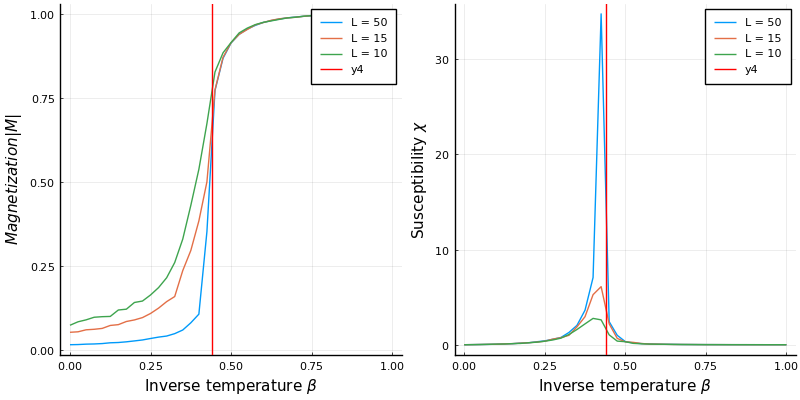
   $M$ : magnetization, a particle spin up $1$ else $-1$

   $\chi$ : susceptibility, $\chi=\frac{\partial M}{\partial H}= \text{Var}(M)\beta$

   $\beta$ : inverse temperature, $\beta = \frac{1}{T\kappa_B}$

2. How to apply M(RT)$^2$ algorithm to Ising Model

   • randomly choose configuration $X_i$
   • compute $\Delta E=E(Y)-E(X)=2J\sigma_i\sigma_j$
   • $A(X\to Y) = \text{min}\left(1,exp(-\frac{\Delta E}{\kappa_BT})\right)$

3. What is the critical temperature for Ising Model ?

   $T_c = \frac{2}{\text{log}(1+\sqrt{2})}$

6. Finite Difference

Error Estimation

1. How many kinds of errors can be categorized?

   • input data error
   • computational rounding error : float point
   • truncation error : infinite term/linear approximation
   • mathematical model error : flawless assumption
   • human&machine error

2. Are mathematically equivalent formulas also numerically equivalent? why?

   no, for example $|(1+\frac{1}{n})^n-e|$ and $|\text{exp}(n\text{log}(1+\frac{1}{n}))-e|$

3. What is error propagation? How to compute it?

   $$|\Delta f|\lesssim \sum_{i=1}^n\left|\frac{\partial f}{\partial x_i}\right||x_i|$$

4. What is ill-conditioned and well-conditioned ?

   ill-conditioned : small changes in the input data can result in large changes in the output data

   well-conditioned : small changes in the input data only result in small changes in the output data

Discretization in Space and Time

1. What’s the parabolic/hyperbolic/elliptic form?
   • parabolic: $D\frac{\partial^2 \phi}{\partial x^2} - \frac{\partial \phi}{\partial t}=0$
   • hyperbolic: $\frac{\partial^2 \phi}{\partial x^2}-\frac{1}{c}\frac{\partial^2 \phi}{\partial t^2} = 0$
   • elliptic: $\nabla^2 \phi = 0$

FTBS

1. What is Forward in Time, Backward in Space?

   $$\begin{aligned} \frac{\partial \phi}{\partial t}&=\frac{\phi_j^{n+1}-\phi_j^n}{\Delta t} +\mathcal O(\Delta t)\\ \frac{\partial \phi}{\partial x}&=\frac{\phi_j^n-\phi_{j-1}^n}{\Delta x}+\mathcal O(\Delta x) \end{aligned}$$

2. What is the order of accuracy for FTBS?

   first order accuracy

3. Assume $c=\frac{u\Delta x}{\Delta t}$, when is FTBS stable and when is it unstable?

   the Domain of Dependence(DoD) for FTBS is $c\in[0,1]$, within the DoD the domain is stable.

4. Solving the linear advection condition $\phi_t+u\phi_x=0$ with FTBS, what is the $|A|^2$ in Von-Neumann Stability?

   $$\begin{aligned} \phi_j^n &= A^n e^{ikj\Delta x} \\ A &= 1-c(1-e^{-ik\Delta x}) \\ |A|^2 &= 1-2c(1-c)(1-cos k\Delta x) \end{aligned}$$

FTCS

1. What is Forward in Time Center in Space ?

   $$\begin{aligned} \frac{\partial \phi}{\partial t}&=\frac{\phi^{n+1}-\phi^{n}}{\Delta t} +\mathcal O(\Delta t)\\ \frac{\partial \phi}{\partial x}&=\frac{\phi_{j+1}-\phi_{j-1}}{\Delta x}+\mathcal O(\Delta x^2) \end{aligned}$$

2. Solving the linear advection condition $\phi_t+u\phi_x=0$ with FTCS, what is the $|A|^2$ in Von-Neumann Stability? What’s different from FTCS?

   $$|A|^2 = 1+4c^2 \text{sin}^2(k\Delta x)$$

CTCS

1. What is Centred in Time, Centred in Space ?

   $$\begin{aligned} \frac{\partial \phi^n_j}{\partial t} &= \frac{\phi_j^{n+1}-\phi_j^{n-1}}{2\Delta t}+\mathcal O(\Delta t^2) \\ \frac{\partial \phi_j^n}{\partial x} &= \frac{\phi_{j+1}^n-\phi_{j-1}^n}{2\Delta x} +\mathcal O(\Delta x^2) \end{aligned}$$

2. How to get the second term $\phi^1$

   use FTCS

3. Assume $c=\frac{u\Delta x}{\Delta t}$, when is CTCS stable and when is it unstable?

   The DoD for CTCS is $c\in[-1,1]$, within the DoD, it’s stable.

4. Solving the linear advection condition $\phi_t+u\phi_x=0$ with CTCS, what is the $|A|^2$ in Von-Neumann Stability? What’s different from FTBS?

   $$A = -ic \text{sin}k\Delta x \pm\sqrt{1-c^2sin^2k\Delta x}$$

   • The solution is stable and not damping since $|A|^2=1\Leftrightarrow |c|\le 1$
   • There are two solutions, one is spurious computational mode, one is the realistic solution

BTCS

1. What is Backward in Time, Centred in Space?

   $$\begin{aligned} \frac{\partial \phi^{n+1}_j}{\partial t} &= \frac{\phi_j^{n+1}-\phi_j^{n}}{\Delta t}+\mathcal O(\Delta t) \\ \frac{\partial \phi_j^{n+1}}{\partial x} &= \frac{\phi_{j+1}^{n+1}-\phi_{j-1}^{n+1}}{2\Delta x} +\mathcal O(\Delta x^2) \end{aligned}$$

2. Is BTCS implicit?

   yes

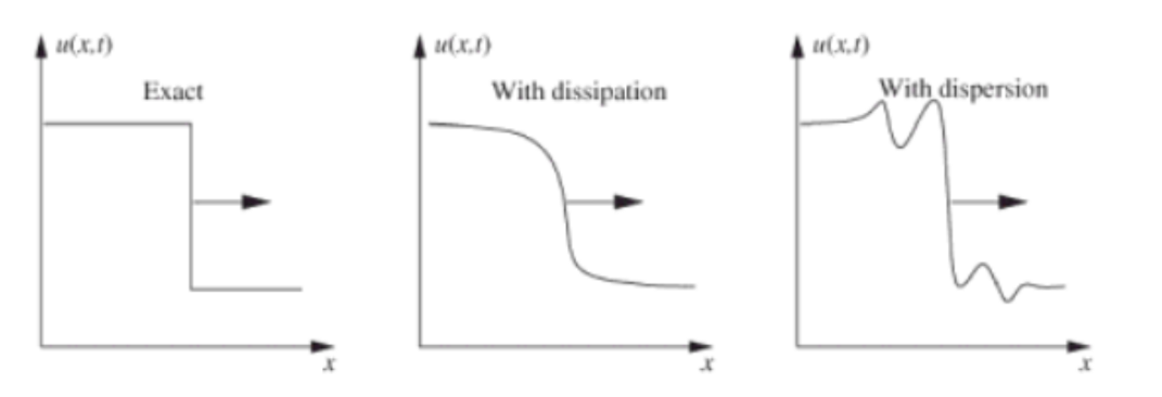
Numerical Analysis

1. What is Numerical diffusion and Numerical dispersion?

   Numerical diffusion: smooth out sharp corners

   Numerical dispersion: Fourier components travel at different speeds

   

2. What is Lax-Equivalence Theorem?

   $$\text{consistency}+\text{stability}\Leftrightarrow \text{convergence}$$

3. What is Courant-Friedrichs-Lewy(CFL) criterion? What’s the CFT condition for linear advection $\phi_t +u\phi_x = 0$?

   $$C = \frac{u\Delta t}{\Delta x}\le C_{max}$$

4. What’s the typical $C_{max}$ for explicit method and implicit method?

   $C_{max}=1$ for explicit method, $C_{max}>1$ for implicit method

5. What is Von-Neumann Stability Analysis?

   $$\phi^{n+1}=A\phi^n\quad A\in \mathbb C$$

   condition	behavior
   $|A|^2<1$	stable and damping
   $|A|^2=1$	neutral stable
   $|A|^2 > 1$	unstable and amplyfying

Phase velocity

1. What is the phase velocity in linear advection $\phi_t+u\phi_x = 0$?

   $u$ since $\phi(x,t)=\phi(x-ut,0)$

2. What is the amplification factor $A$ of linear advection analytical solution?

   $A=e^{-iku\Delta t}$

3. What is the phase speed for amplification factor $e^{-i\alpha}$ with wave number $K$?

   $\alpha/(k\Delta t)$

4. What is the amplification factor of CTCS?

   $$A = -ic\text{sin}k\Delta x\pm\sqrt{1-c^2 \text{sin}^2k\Delta x}$$

5. What is the phase speed $u_n$ in linear advection when using CTCS method? What phenomenon do you observe?

   

   $$u_n = \frac{1}{k\Delta t}\text{tan}^{-1}\frac{c\text{sin}k\Delta x}{\pm\sqrt{1-c^2\text{sin}^2k\Delta x}} =\pm\frac{\text{sin}k\Delta x}{k\Delta x}u$$

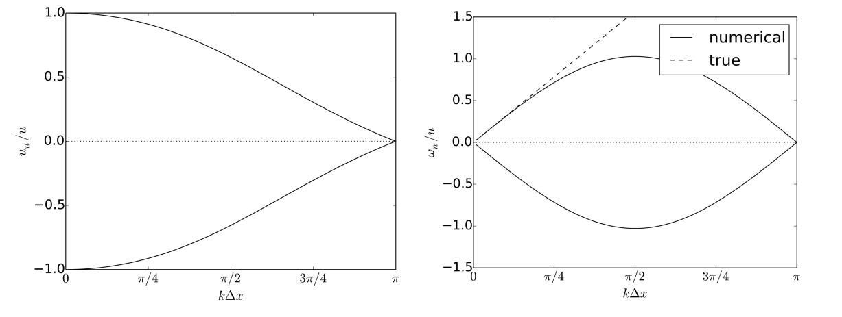
   • There are two solutions, the positive one is the physical mode.
   • The physical mode is close to the ground truth when $k$ and $\Delta x$ is very small.

Shallow water equation

1. What is the equation for incompressible navier stokes?

   $$\begin{aligned} \frac{\partial v}{\partial t} + (v\cdot \nabla) v &= -\frac{1}{\rho}\nabla p + g \\ \nabla\cdot v &= 0 \end{aligned}$$

2. Assume the gravity only in $z$ direction, what PDE equation can we get from the incompressible navier stokes? How about 1D condition?

   $$\begin{aligned} \frac{\partial H'}{\partial t} &= -H_0\left(\frac{\partial \int_{-H^0}^{H'} v_x dz}{\partial x}+\frac{\partial \int_{-H^0}^{H'} v_y dz}{\partial y}\right) \\ \frac{\partial \int_{-H^0}^{H'} v_x dz}{\partial t} &= -g \frac{\partial H'}{\partial x} \\ \frac{\partial \int_{-H^0}^{H'} v_y dz}{\partial t}&=-g\frac{\partial H'}{\partial y} \end{aligned}$$

   1 D condition

   $$\begin{aligned} \frac{\partial H'}{\partial t} &= -H_0\frac{\partial \int_{-H^0}^{H'} v_x dz}{\partial x} \\ \frac{\partial \int_{-H^0}^{H'} v_x dz}{\partial t} &= -g \frac{\partial H'}{\partial x} \end{aligned}$$

3. In 1 D wave condition, assume $u= \int_{-H^0}^{H'}v_x dz$ and $\eta=H'$, give the unstaggered(A-grid) and staggered(C-grid) formular of centered in space. Assume $c = \sqrt{gH_0}\frac{\Delta t}{\Delta x}$, what are the stable conditions for them?

   

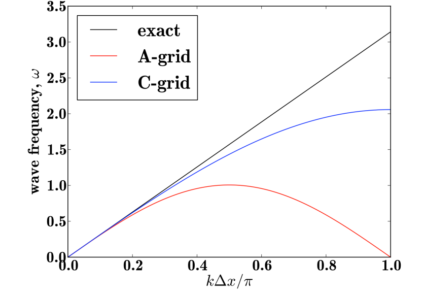
   A-grid

   stable for $c\le 2$

   $$\frac{\eta^n_j - \eta^{n-1}_j}{\Delta t} = - H_0 \frac{u^n_{j+1} - u^n_{j-1}}{\Delta x} \\ \frac{u^{n+1}_j - u^n_j}{\Delta t} = -g \frac{\eta^n_{j+1} - \eta^n_{j-1}}{\Delta x}$$

   C-grid

   stable for $c\le 1$

   better at high frequency

   $$\frac{\eta_j^n- \eta^{n-1}_j}{\Delta t} = - H_0\frac{u^n_{j+\frac{1}{2}}-u^n_{j-1}}{\Delta x} \\ \frac{u^{n+1}_{j+\frac{1}{2}} - u^n_{j+\frac{1}{2}}}{\Delta t} = - g \frac{\eta^n_{j+1} - \eta^n_{j-1}}{\Delta x}$$

7. Time Integration

Error

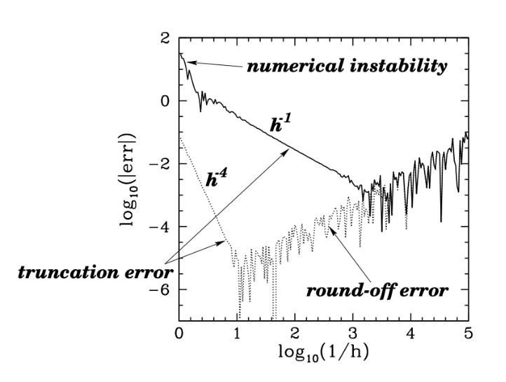
1. What’s the difference between truncation error and round-off error?

   Truncation error results from Taylor expansion

   Roundoff error results from the float point computation

2. What is the round off error for explicit euler of timestep $\Delta t$?

   $\mathcal O\left(\frac{\eta}{\Delta t}\right)$ where $\eta=\text{eps}(\text{float})$

3. What is the truncation error for explicit euler of timestep $\Delta t$?

   $\mathcal O(\Delta t)$

4. What are the two main drawbacks of explicit euler compared to rounge kutta method?

   • it’s numerical instable
   • it has first order of truncation error which is lager then rounge kutta

5. Describe the picture below.

   

Conservation

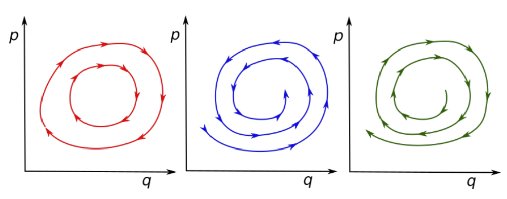
1. What is Symplectic?

   $|\text{det}(A)|=1$

2. Given Hamitonian transformation $A=\begin{bmatrix}\text{cos}\tau&\text{sin}\tau\\-\text{sin}\tau&\text{cos}\tau\end{bmatrix}$ that $\begin{bmatrix}q'\\p'\end{bmatrix}=A\begin{bmatrix}q\\p\end{bmatrix}$, what is the modified Hamitoninan transformation for the first order of $\tilde A$?

   $\begin{bmatrix}1&\tau\\-\tau&1-\tau^2\end{bmatrix}$

3. Describe the picture below from the conservation view.

   

8. Maxwell Equation

1. Give the general formula of Vlasov-Maxwell-Boltzmann equation describing the plasma distribution $f(\textbf{x},\textbf{v},t)\in \R^{3\times 3\times 1}$.

   $$\begin{aligned} \frac{\partial f}{\partial t} &+ \nabla_\textbf{x} \cdot(\textbf{v}f) + \nabla_\textbf{v}\cdot (\textbf{F}f) = \left(\frac{\partial f}{\partial t}\right)_c \\ \textbf F &= \frac{q}{m(\textbf{E}+\textbf{v}\times \textbf{B})} \end{aligned}$$

   $\nabla_\textbf{x}\cdot (\textbf{v}f)$ : advection in real space

   $\nabla_\textbf{v}\cdot (\textbf{F}f)$ : advection in velocity space

   $\textbf F = \frac{q}{m(\textbf{E}+\textbf{v}\times \textbf{B})}$ : lorentz force

   $\left(\frac{\partial f}{\partial t}\right)_c$:collision term, normally $0$ in Vlasov equation

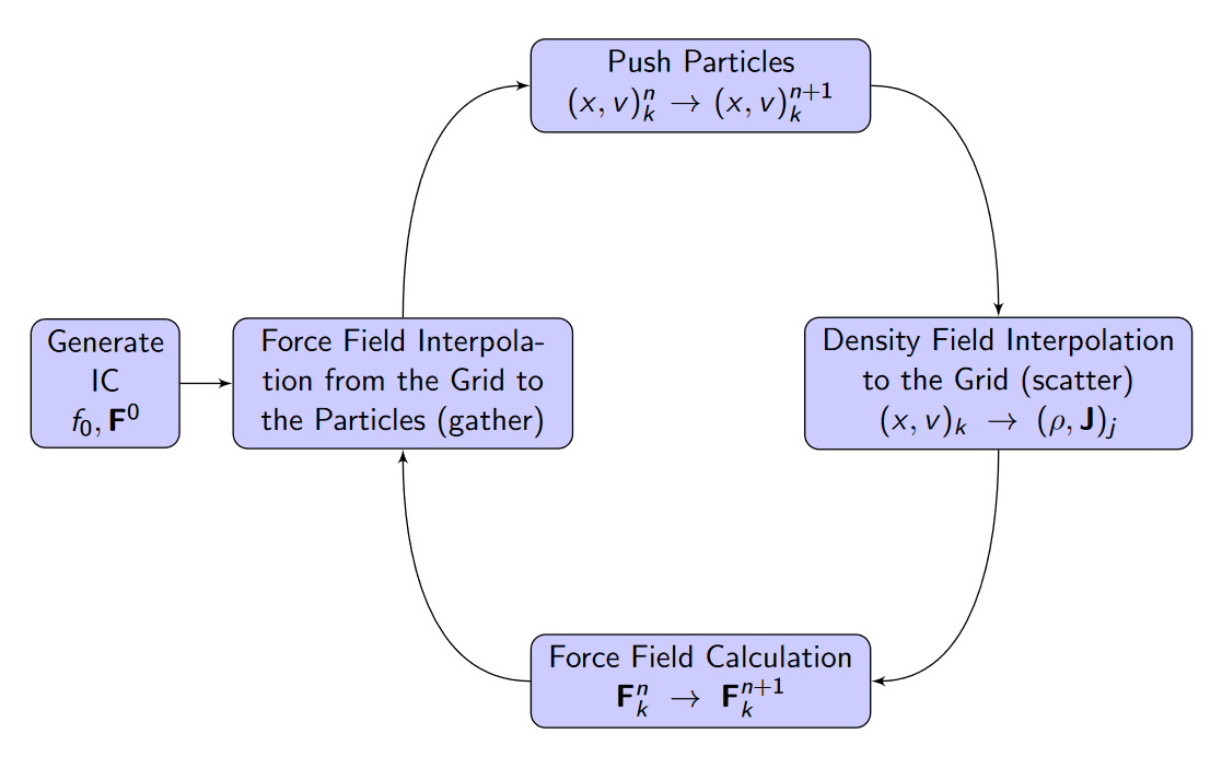
particle in cell

1. Describe the Particle in Cell(PIC) method.

   $$\begin{aligned} \frac{d\boldsymbol x}{dt} &= \boldsymbol v\\ \frac{d\boldsymbol v}{dt} &= \frac{q}{m}(\boldsymbol E(\boldsymbol x,t), \boldsymbol v\times \boldsymbol B(\boldsymbol x, t)) \end{aligned}$$

   

Boris Algorithm

1. Describe the Boris Algorithm.

   $$\begin{aligned} \textbf{v}^- &= \textbf{v}^{n-\frac{1}{2}} + \frac{q}{m} \boldsymbol E^n\frac{\Delta t}{2} \\ \textbf{t} &= \text{tan}\left(\frac{qB\Delta t}{2m}\right)\frac{\textbf{B}}{B} \approx \frac{q\textbf{B}\Delta t}{2m} \\ \textbf{s} &= \frac{2t}{1+|t|^2} \\ \textbf{v}' &= \textbf{v}^-+\textbf{v}^-\times\textbf{t} \\ \textbf{v}^+ &= \textbf{v}^- + \textbf{v}'\times \textbf{s} \\ \textbf{v}^{n+\frac{1}{2}} &= \textbf{v}^+ + \frac{q}{m}\boldsymbol E^n\frac{\Delta t}{2} \end{aligned}$$

2. Show what the absence of $\textbf{E}$ of the Boris algorithm conserves kinetic energy.

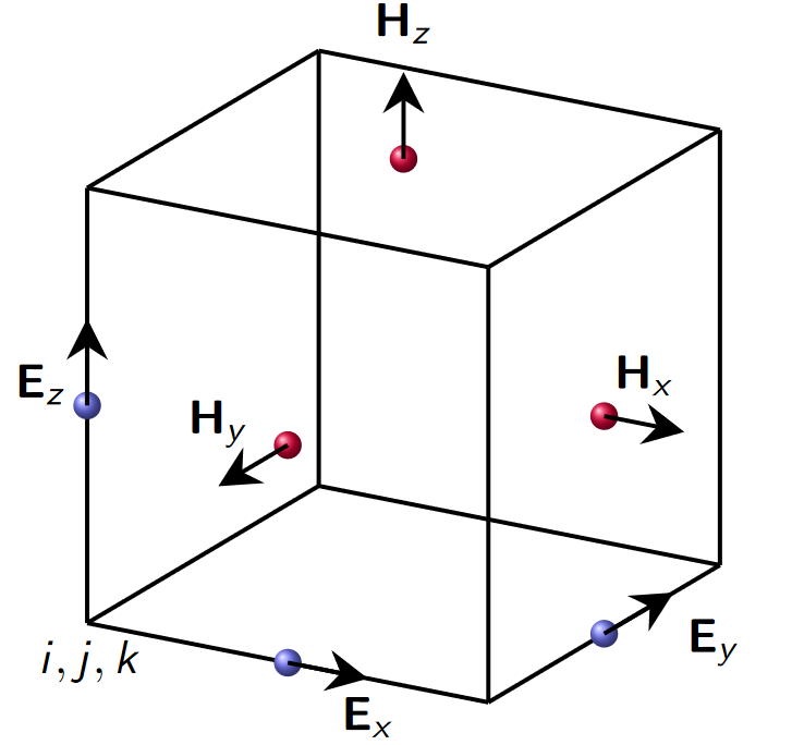
Yee-cell

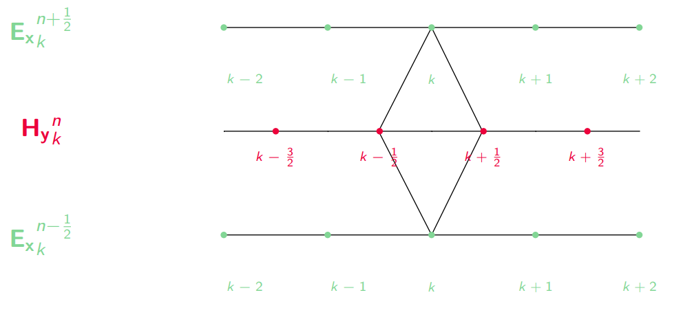
1. Describe the Yee-Cell method.

   

   $$\frac{E_{x_k}^{n+\frac{1}{2}}-E_{x_k}^{n-\frac{1}{2}}}{\Delta t} = -\frac{1}{\varepsilon_0}\frac{H_{y_{k+\frac{1}{2}}}^n - H_{y_{k-\frac{1}{2}}}^n}{\Delta z} \\ \frac{H_{y_{k+\frac{1}{2}}}^{n+1}-H_{y_{k+\frac{1}{2}}}^n}{\Delta t} = -\frac{1}{\mu_0}\frac{E_{x_{k+1}}^{n+\frac{1}{2}}-E_{x_k}^{n+\frac{1}{2}}}{\Delta z}$$

   

2. How to determine the time step $\Delta t$?

   $\Delta t = \frac{\Delta x}{\sqrt{d}c}$ where $d$ is dimension

3. How to minimize the error of by scaling $E_x$ ?

   $\tilde E_x = \sqrt{\frac{\varepsilon_0}{\mu_0}}E_x$

9. Nbody Problem

1. List some algorithm to solve n-body problem numerically.
   • PIC(Particle in Cell) : grid field solver
   • P3M(Particle-particle Particle-Mesh) : split forces into short and long range
   • Langevin : using Rosenbluth potentials
   • SPH(Smooth Particle Hydrodynamics) : between finite sized
   • FMM(Fast multipole method) : use center of force
   • Tree Methods : mesh free

PIC(Particle In Cell)

P3M(Particle-Particle Particle-Mesh)

1. Describe the general idea of P3M algorithm.
   • nearby particles - nbody calculation $\mathcal O(n^2)$
   • fa away particles - PIC algorithm $\mathcal O(n)$