Mathematics for New Technologies in Finance

MNTF Mathematics for New Technologies in Finance

professor : Josef Teichmann

author : walkerchi


Approximation

Weierstrass

Weierstrass Approximation Theorem

AA is dense in C(X,Rm)={fi∣fi∈Cpw0,fi∈X→Rm,X⊂Rn}C(\mathcal X,\R^m )=\{f_i|f_i\in C_{pw}^0, f_i\in \mathcal X\to \R^m,\mathcal X\subset \R^n\} if

  1. A contains all polynomial functions: P⊂A\mathcal P\subset A
    1. AA is vector subspace of CC : $A\subset C(\mathcal X,\R^m)\quad $
      • f1(x)+f2(x)=f3(x)∀f1,f2∈A,∃f3∈Af_1(x)+f_2(x)=f_3(x)\quad \forall f_1,f_2\in A,\exists f_3\in A
      • cf1(x)=f2(x)∀c∈R,∀f1∈A,∃f2∈Acf_1(x)=f_2(x)\quad \forall c\in\R,\forall f_1\in A,\exists f_2\in A
    2. AA is closed under multiplication : f1(x)f2(x)=f3(x)∀f1,f2∈A,∃f3∈Af_1(x)f_2(x)=f_3(x)\quad \forall f_1,f_2\in A,\exists f_3\in A
    3. AA contains constant function : f(v)=c∀v∈X,∃f∈Af(v) = c\quad \forall v\in \mathcal X,\exists f\in A
  2. points seperation : f(v)\neq f(w)\quad \forall v\neq w\and v,w\in\mathcal X

for shallow NN with ReLU

  • [ ] contains all polynomial functions
    • [ ] vector space
    • [ ] closed under multiplication
    • [x] contains constant function
  • [x] points seperation

⇒\Rightarrow NN with ReLU is dense in C(X,Rm)C(\mathcal X,\R^m)

Faber-Schauder

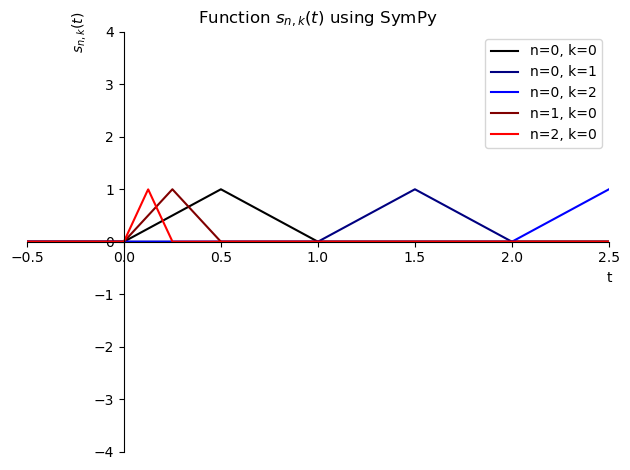
Faber-Schauder basis : sn,k=21+n2∫0tψn,k(u)dun,k∈Zs_{n,k} = 2^{1+\frac{n}{2}}\int_0^t\psi_{n,k}(u)\text du\quad n,k\in\Z

faber schauder basis

v=∑n=0∞αnbn∀v∈R,∃αn∈R,∃bn∈{s∗,∗}v = \sum_{n=0}^\infin \alpha_n b_n\quad \forall v\in \mathbb R,\exists\alpha_n\in\mathbb R,\exists b_n\in \{s_{*,*}\}

  • equivalent to the linear combination of ReLU

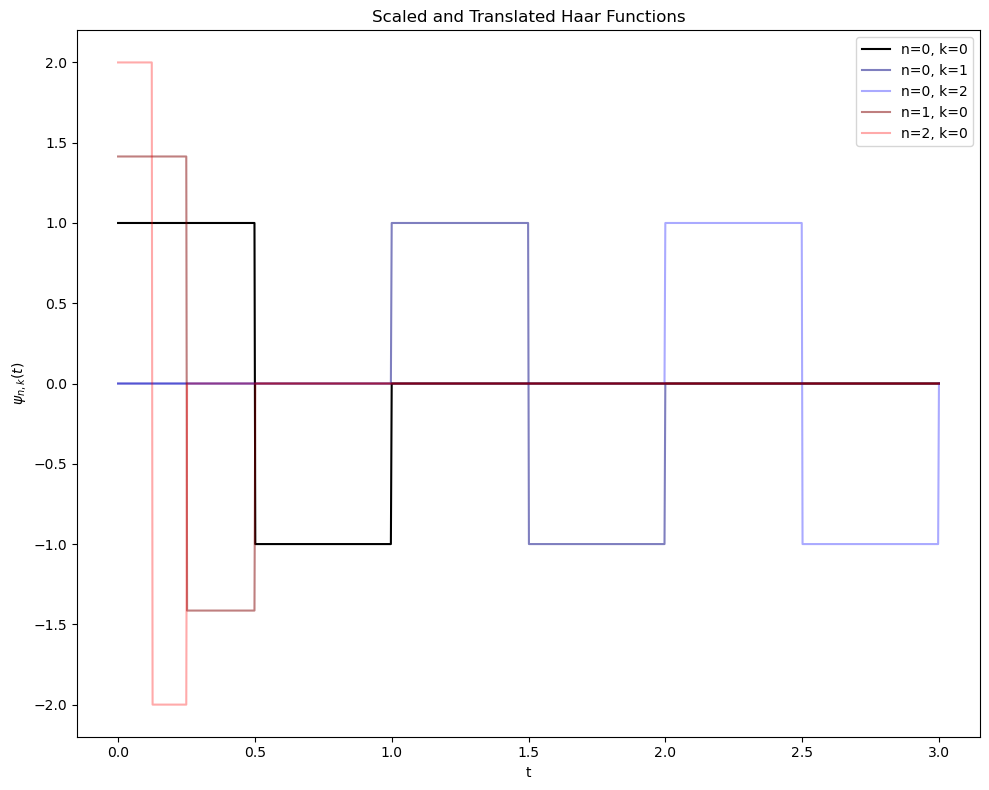
Haar function : ψn,k(t)=2n/2ψ(2nt−k)n,k∈Zψ(t)={1t∈[0,12)−1t∈[12,1)0otherwise\psi_{n,k}(t) =2^{n/2}\psi(2^nt-k)\quad n,k\in \Z\quad\psi(t) = \begin{cases}1&t\in[0, \frac{1}{2})\\-1&t\in[\frac{1}{2},1)\\ 0&\text{otherwise}\end{cases}

haar function

  • supp(ψn,k)=[k2−n,(k+1)2−n)\text{supp}(\psi_{n,k}) = [k2^{-n},(k+1)2^{-n})
  • ∫Rψn,k(t)dt=0\int_\R \psi_{n,k}(t)\text dt = 0
  • ∥ψn,k∥L2(R)=1\Vert \psi_{n,k}\Vert_{L^2(\R)} = 1
  • ∫Rψn1,k1ψn2,k2dt=δn1n2δk1k2\int_\R \psi_{n_1,k_1}\psi_{n_2,k_2} \text d t=\delta_{n_1n_2}\delta_{k_1k_2}

Banach

AA is Banach space if :

  1. Cauchy sequence : ∥fm−fn∥≤ϵ∀ϵ>0,∃Nϵ∈N,∀m,n>Nϵ\Vert f_m-f_n\Vert\le \epsilon\quad \forall \epsilon>0,\exists N_\epsilon\in \N,\forall m,n>N_\epsilon
  2. completeness : ∥f−fm∥≤ϵ∀ϵ>0,m→∞\Vert f-f_m\Vert\le \epsilon \quad \forall \epsilon>0, m\to\infin

Signature

for path/curve Xt∈RdX_t\in \R^d, Xt=[X1(t)X2(t)⋯Xd(t)]⊤X_t=\begin{bmatrix}X^1(t)&X^2(t)&\cdots&X^d(t)\end{bmatrix}^\top , signature could determine the curve in tree like equivalences

n-th level of signature : S(X)a,bi1,i2,⋯ ,in=∫ab∫atn−1⋯∫at2dXt1i1⋯dXtninn≤dS(X)_{a,b}^{i_1,i_2,\cdots,i_n}=\int_a^b\int_{a}^{t_{n-1}}\cdots \int_a^{t_2}\text dX_{t_1}^{i_1}\cdots \text dX_{t_n}^{i_n}\quad n \le d

  • S(X)a,bi1,i2,⋯ ,in∈Rn⊗dS(X)_{a,b}^{i_1,i_2,\cdots,i_n}\in \R^{n^{\otimes d}}, it’s a dd dimension tensor with each dimension of span nn

signature : S(X)a,b=(1,S(X)a,bi1,S(X)a,bi1,i2,⋯ ,S(X)a,bi1,i2,⋯ ,id)S(X)_{a,b} = (1,S(X)_{a,b}^{i_1},S(X)_{a,b}^{i_1,i_2},\cdots,S(X)_{a,b}^{i_1,i_2,\cdots,i_d})

  • the maximum length of S(X)a,bS(X)_{a,b} is d0+d1+d2+⋯+dd=dd+1−1d−1d^0+d^1+d^2 + \cdots + d^d = \frac{d^{d+1}-1}{d-1}
  • the length of depth MM is d0+⋯+dM=dM+1−1d−1d^0 + \cdots +d^{M} = \frac{d^{M+1} - 1}{d-1}

normally we got : XaiX_a^i denotes ii-th component at time aa of vector of function XX

  • S(X)a,bi=∫abdX=Xbi−XaiS(X)_{a,b}^i = \int_a^b dX = X_b^i-X_a^i

  • S(X)a,bi,j=∫ab∫at2dXt1idXt2j=∫ab(Xt2i−Xai)dXt2j=X=αt+β12(Xbi−Xai)(Xbj−Xaj)S(X)_{a,b}^{i,j} = \int_a^b\int_a^{t_2}dX_{t_1}^{i}dX_{t_2}^{j} =\int_a^b (X_{t_2}^i-X_a^i)dX_{t_2}^j\overset{X=\alpha t+\beta}{=} \frac{1}{2}(X_b^{i}-X_a^{i})(X_b^{j}-X_a^{j})

  • S(X)a,bi,j,k=∫ab∫at3∫at2dXt1idXt2jdXt3k=X=αt+β16(Xbi−Xai)(Xbj−Xaj)(Xbk−Xak)S(X)_{a,b}^{i,j,k} = \int_a^b\int_a^{t_3}\int_a^{t_2}dX_{t_1}^{i}dX_{t_2}^{j}dX_{t_3}^{k} \overset{X=\alpha t+\beta}{=} \frac{1}{6}(X_b^{i}-X_a^{i})(X_b^{j}-X_a^{j})(X_b^{k}-X_a^{k})

  • shuffle product rule : S(X)a,bIS(X)a,bJ=∑K=shuff([I1,⋯ ,J1,⋯ ])S(X)a,bKS(X)_{a,b}^IS(X)_{a,b}^J = \underset{K=\text{shuff}([I_1,\cdots,J_1,\cdots])}{\sum}S(X)_{a,b}^K

    • example : S(X)a,b1S(X)a,b2=S(X)a,b1,2+S(X)a,b2,1S(X)^{1}_{a,b} S(X)^2_{a,b} = S(X)^{1,2}_{a,b}+S(X)^{2,1}_{a,b}

Financial Market

Notation

  • StiS_t^i : ii-th asset prices at time tt, S∈RN×d+1S\in\R^{N\times {d+1}}, normally S0S^0 represent bank account
  • ϕti\phi_t^i : holdings/strategy in ii-th assets at time tt
  • VtV_t : value of portfolio at time tt , Vt=∑iϕtiStiV_t = \sum_i \phi_t^i S_t^i

self-financing : dV(t)=∑i=1nϕi(t)dSi(t)\text dV(t) = \sum_{i=1}^n \phi^i(t)\text dS^i(t)

  • ∑iϕt+1iSti=∑iϕtiSti∀t∈[0,N)\sum_i \phi^i_{t+1}S_t^i = \sum_i\phi_t^i S_t^i\quad\forall t\in[0,N)

value process : Vt+1−Vt=∑iϕti(St+1i−Sti)∀t∈[0,N)V_{t+1}-V_t = \sum_i\phi_t^i(S_{t+1}^i-S_t^i)\quad \forall t\in[0,N)

martingale : E[Xn+1∣X1,…,Xn]=Xn\mathbb E[X_{n+1}|X_1,\dots,X_n] = X_n

arbitrage : P(Vt≥0)=1⏟no risk of losing money∧P(Vt≠0)>0⏟portfolio value > 0t∈(0,T),V0=0⏟requires no initial value\underbrace{P(V_t\ge 0 )=1}_{\text{no risk of losing money}}\land \underbrace{P(V_t\neq 0) >0}_{\text{portfolio value > 0}}\quad t\in (0,T),\underbrace{V_0=0}_{\text{requires no initial value}}

Stochastic Differential Equation

Brownian motion/Wiener process : Wt+1−Wt∼N(0,1)W0=0→WtW_{t+1} - W_t \sim \mathcal N(0,1)\quad W_0=0\rightarrow W_t

Geometric Brownian motion : dSt=μ St dt+σ St dWt⇔St=S0e(μ−σ22)t+σWtdS_t = \mu ~S_t~ dt + \sigma~ S_t~ dW_t\Leftrightarrow S_t = S_0 e^{\left(\mu - \frac{\sigma^2}{2}\right)t+\sigma W_t}

  • WtW_t is brownian motion/wiener process
  • μ,σ\mu,\sigma is the expectation/variance for the GBM
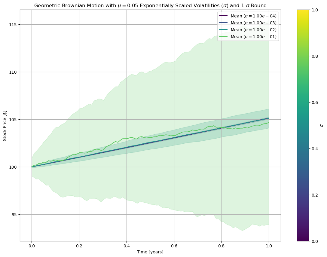
geometric brownian motion

Utility

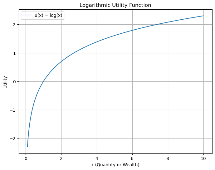
utility function uu : the additional utility or satisfaction from consuming one more unit of a good decreases as more of the good is consumed.

  • concave : f′′(x)<0f''(x)<0
  • monotone increase : f′(x)>0f'(x)>0
img

expected utility optimization problem : argmaxϕti E[u(VN)]\underset{\phi_t^i}{\text{argmax}}\mathbb~E[u(V_N)]

Local Volatility Model : dSt=rStdt+σ(St,t)StdWt\text d S_t = rS_t\text d t+\sigma(S_t,t)S_t\text dW_t

  • StS_t : underlying asset price at time tt

  • rr risk-free interesting rate

  • σ(St,t)\sigma(S_t,t) : local volatility function

  • WtW_t is the Brownian motion/ Wiener process

Local Stochastic volatility model : dSt=μStdt+νtStdWtdνt=αt(ν)dt+βt(ν)dWt′\begin{aligned}\text d S_t &= \mu S_t \text d t+\sqrt{\nu_t} S_t \text dW_t\\ \text d\nu_t &= \alpha_{t}(\nu)\text dt + \beta_{t}(\nu)\text d W'_t\end{aligned}

  • αt(ν),βt(ν)\alpha_{t}(\nu),\beta_{t}(\nu) : functions based on ν\nu
  • Wt,Wt′W_t,W'_t : Wiener process with correlation factor ρ\rho
  • νt\nu_t : model the variance of StS_t, it relies on another stochastic process, so LSV is not a standard SDE

Heston model : dνt=κ(θ−νt)dt+ξνtdWt′\text d\nu_t = \kappa(\theta-\nu_t)\text dt +\xi \sqrt{\nu_t}\text d W'_t

  • θ\theta : long term variance

  • κ\kappa : rate of variance reverts toward it’s long term

  • ξ\xi : volatility of volatility, the variance of νt\nu_t

  • ambitious approach

    • modeling θ,κ,ξ,ρ,μ\theta,\kappa,\xi,\rho,\mu where ρ\rho is the correlation between Wt,Wt′W_t,W'_t
  • modest approach

    • modeling θ,κ,ξ\theta, \kappa,\xi , and ρ,μ\rho,\mu from emperical

Ito’s lemma : df(S,t)=(∂f∂t+μ∂f∂S+12σ2∂2f∂S2)dt+σ∂f∂SdWtdS(t)=μdt+σdWt⏟Stochastic Differential Equation\text d f(S,t) = \left(\frac{\partial f}{\partial t} + \mu\frac{\partial f}{\partial S}+\frac{1}{2}\sigma^2\frac{\partial^2 f}{\partial S^2}\right)\text dt + \sigma\frac{\partial f}{\partial S}\text dW_t\quad \underbrace{\text dS(t)=\mu \text dt+\sigma \text d W_t}_{\text{Stochastic Differential Equation}}

Black Scholes equation : ∂C∂t+rK∂C∂K+12σ2K2∂2C∂K2−rC=0\frac{\partial C}{\partial t} + rK\frac{\partial C}{\partial K} +\frac{1}{2}\sigma^2 K^2\frac{\partial^2 C}{\partial K^2}-rC= 0 : derive from Ito’s lemma

  • C(K,t)C(K,t) : European call option price, equivalent to value VV
  • KK : strike price, equivalent to assets/stock price SS

Dupire’s formula : −∂C∂T−rK∂C∂K+12σ2K2∂2C∂K2−ΔC=0-\frac{\partial C}{\partial T}-rK\frac{\partial C}{\partial K}+\frac{1}{2}\sigma^2K^2\frac{\partial^2 C}{\partial K^2}-\Delta C=0

  • when r=0r=0 , σ2=2∂TCK2∂K2C\sigma^2 = \frac{2\partial_T C}{K^2\partial^2_K C}

Breeden-Litzenberger fromula : ∂K2C(T,K)dK=pT(K)dK\partial^2_K C(T,K)\text dK = p_T(K)\text d K

  • pT(K)dKp_T(K)\text dK is the risk neural probability, pT(K)=p(St∈[K,K+dK])p_T(K) = p(S_t\in[K,K+\text dK])

Deep portfolio optimization

dSt=Stμdt+StσdWtdXt=αtXtdStSt+(1−α)Xtrdtmaxα E[u(XT)]\text d S_t = S_t\mu \text d t+S_t\sigma\text d W_t \\ \text dX_t = \alpha_t X_t\frac{\text dS_t}{S_t} + (1-\alpha) X_t r\text dt\quad \\ \underset{\alpha}{\text{max}}~\mathbb E[u(X_T)]

  • XtX_t is the money at time tt
  • αt\alpha_t is strategy how much portion of money in the stock rather than in the bank at time tt
  • StS_t is the stocks prices, governed by parameter μ\mu and σ\sigma , with WtW_t a brownian motion or wiener process
  • rr is the interest rate saved in bank
  • uu is the utility function ,normally u(x)=xγ−1γu(x)=\frac{x^\gamma -1}{\gamma}

analytical solution : α∗=μ−rσ2(1−γ)\alpha^* = \frac{\mu-r}{\sigma^2(1-\gamma)}


Deep Hedging

dSt=Stμdt+StσdWtminH,π E[∥f(ST)−π−∫0THtdSt∥2]\text d S_t = S_t\mu \text d t+S_t\sigma\text d W_t \\ \underset{H,\pi}{\text{min}}~\mathbb E\left[\left\Vert f(S_T) - \pi - \int_0^T H_t\text dS_t\right\Vert^2\right]

  • StS_t is the risky stocks prices, governed by parameter μ\mu and σ\sigma , with WtW_t a brownian motion or wiener process
  • f(St)f(S_t) is financial claim, the payoff is f(ST)=max(ST−K,0)f(S_T)=\text{max}(S_T-K,0) for European call, KK is the strike price
  • π\pi the price of the option, the upfront payment you received
  • HtH_t is the hedge strategy at time tt
  • TT is the expire date

Deep Calibration

Heston Calibration

dXt=((q−r)−12Yt)dt+YtdWt1dYt=(θ−κYt)dt+σYtdWt2argminθ,κ,σ∑t=0T∥Xt−log(St)∥2\text dX_t = \left((q-r)-\frac{1}{2}Y_t\right)\text d t +\sqrt {Y_t}\text d W_t^1 \\ \text dY_t = (\theta-\kappa Y_t)\text d t +\sigma\sqrt{Y_t}\text dW^2_t \\ \underset{\theta,\kappa,\sigma}{\text{argmin}}\sum_{t=0}^T\Vert X_t-\text {log}(S_t)\Vert^2

  • rr : interest rate
  • qq : dividend
  • StS_t : price of assets
  • XtX_t : predicted log price : X0=log(S0)X_0 = \text{log}(S_0)
  • YtY_t : variance of Heston model : Y0=ν0Y_0 = \nu_0

Utility Calibration

dSt=Stαtl(t,St)dWtargminl∥E[max(ST−K,0)−C(K,T)−∫0THtdSt]∥2dS_t = S_t\alpha_t l(t,S_t)\text dW_t \\ \underset{l}{\text{argmin}} \left\Vert\mathbb E\left[\text{max}(S_T-K,0) - C(K,T)- \int_0^T H_t\text dS_t\right]\right\Vert^2

  • αt\alpha_t is exogenous process at time
  • l(t,St)l(t, S_t) is leverage function
  • StS_t is the stocks prices, with WtW_t a brownian motion or wiener process
  • HtH_t is the hedge strategy at time tt
  • KK is the strike price of European call
  • CC is the European call option market price

Deep Simulation

model controlled differential equation

dXt=∑i=0dσ(AiXt+bi)dui(t)\text d X_t = \sum_{i=0}^d \sigma(A_iX_t+b_i)\text du_i(t)

  • Ai,biA_i, b_i are randomly generated matrices/vectors
  • uiu_i is control coefficient learned by network
  • σ\sigma is the sigmoid//tanh function

Reinforcement Learning

  • a,sa,s : action a∈Aa\in A, state s∈Ss\in S
  • V,V∗V,V^* : value function, optimal value function, V∈S×T→RV\in S\times T\to\R
  • π(s)\pi(s) : policy , π∈S→A\pi \in S\to A
  • c(t,s,a)c(t,s,a) : cost function , c∈T×S×A→Rc\in T\times S\times A\to \R
  • r,R(s,a)r,R(s,a) : reward, reward function , r∈R,R∈S×A→Rr\in \R, R\in S\times A\to \R
  • Q(s,a)Q(s,a) :Q/state action function, return the priority for each state and action, Q∈S×A→RQ\in S\times A\to \R

[DPP] Dynamic programming principle : V∗(t,s)=maxa{∫tTc(τ,s(τ),a(τ))dτ+V∗(T,s(T))}V^*(t,s)=\underset{a}{\text{max}}\left\{\int_t^T c(\tau,s(\tau),a(\tau))\text d\tau+V*(T,s(T))\right\}

  • V(s)=maxa(R(s,a)+γ∑s′∈SP(s′∣s,a)V(s′))V(s) = \underset{a}{\text{max}}\left(R(s,a)+\gamma\underset{s'\in S}{\sum}P(s'|s,a)V(s')\right)

[HJB] Hamiton-Jacobi-Bellman equation : ∂V(s,t)∂t+maxa(∂V(s,t)∂s⋅f(t,s,a)+c(t,s,a))=0\frac{\partial V(s,t)}{\partial t} + \underset{a}{\text{max}}\left(\frac{\partial V(s,t)}{\partial s}\cdot f(t,s,a)+c(t,s,a)\right)=0

  • f(t,s,a)f(t,s,a) : system dynamics, how state change over time, ds(t)dt=f(t,s,a)\frac{\text d s(t)}{\text dt} = f(t,s,a)
  • V∗(s)=maxa∈A(R(s,a)+γ∑s′∈SP(s′∣s,a)V∗(s′))V^*(s) = \underset{a\in A}{\text{max}} \left(R(s,a)+\gamma \underset{s'\in S}{\sum}P(s'|s,a)V^*(s')\right)

Bellman equation : Q(s,a)=r+γ maxa′ Q(s′,a′)Q(s,a) = r+\gamma~\underset{a'}{\text{max}}~Q(s',a')

Value Iteration : V(n+1)=maxa{R(s,a)+γ∑s′P(s′∣s,a)V(n)(s′)}V^{(n+1)}=\underset{a}{\text{max}}\left\{R(s,a)+\gamma \sum_{s'}P(s'|s,a)V^{(n)}(s')\right\}

Policy Iteration : Vπ(n)(s)=R(s,π(s))+γ∑s′P(s′∣s,π(s))Vπ(n)(s′)π(n+1)=argmaxπ{R(s,a)+γ∑s′P(s′∣s,a)Vπ(n)(s′)}\begin{aligned}V^{\pi^{(n)}}(s) &= R(s,\pi(s))+\gamma\sum_{s'}P(s'|s,\pi(s))V^{\pi^{(n)}}(s')\\\pi^{(n+1)}&=\underset{\pi}{\text{argmax}}\left\{R(s,a)+\gamma\sum_{s'} P(s'|s,a)V^{\pi^{(n)}}(s')\right\}\end{aligned}

Q learning(environment-known/model-based) : Q(s,a)←R(s,a)+∑s′P(s′∣s,a)[γ maxa′ Q(s′,a′)]Q(s,a)\gets R(s,a)+\sum_{s'} P(s'|s,a)\left[\gamma~\underset{a'}{\text{max}}~Q(s',a')\right]

Q learning(environment-unknown/model-free) : Q(s,a)←(1−α)Q(s,a)+α[r+γ maxa′ Q(s′,a′)−Q(s,a)]Q(s,a)\gets (1-\alpha)Q(s,a)+\alpha\left[r+\gamma~\underset{a'}{\text{max}}~Q(s',a')-Q(s,a)\right]


Optimization

inverse calibration : argminθ∥d−NNθ∥2\underset{\theta}{\text{argmin}}\Vert \textbf d - \mathcal {NN}_\theta\Vert^2

  • d\textbf d is the observed data
  • NNθθ∈Θ\mathcal {NN}_\theta\quad \theta\in\Theta is the pool of the model

optimization approach : argminθ∥d−NNθ∥2+λRθ\underset{\theta}{\text{argmin}}\Vert \textbf d-\mathcal{NN}_\theta\Vert^2 + \lambda R_\theta

  • θ\theta model parameters
  • RθR_\theta : regularization term (∣⋅∣|\cdot| : lasso(L1) or ∥⋅∥2\Vert\cdot\Vert^2 : ridge(L2))

bayesian optimization :

P(Mi∣d)=P(d∣Mi)P(Mi)P(d)∝P(d∣Mi)P(Mi)P(M_i|\textbf d) = \frac{P(\textbf d|M_i)P(M_i)}{P(\textbf d)}\propto P(d|M_i)P(M_i)

  • P(Mi∣d)P(M_i|\textbf d) posterior probability of model MiM_i given data d\textbf d
  • P(d∣Mi)P(\textbf d|M_i) likelihood of data given model MiM_i
  • P(Mi)P(M_i) : prior probability of model MiM_i
  • P(d)P(\textbf d) : evidence likelihood

for linear model Y∼N(θX,σ2I),θ∼N(0,τ2I)Y\sim \mathcal N(\theta X,\sigma^2\textbf I), \theta\sim\mathcal N(0,\tau^2\textbf I), the maximizing posterior of p(θ∣x,y)p(\theta|x,y) is ridge regression:

argmaxθ p(θ∣x,y)∝argmaxθ p(θ)p(y∣x,θ)∝argmaxθ exp(−θ⊤Iθ/τ2) exp(−(y−θx)⊤I(y−θx)/σ2)∝argminθ σ2τ2∥θ∥2+∥y−θx∥2\begin{aligned} \underset{\theta}{\text{argmax}} ~p(\theta|x,y) &\propto \underset{\theta}{\text{argmax}}~p(\theta)p(y|x,\theta) \\ &\propto \underset{\theta}{\text{argmax}}~\text{exp}\left(-\theta^\top \textbf I\theta /\tau^2 \right)~\text{exp}\left(-(y-\theta x)^\top \textbf I(y-\theta x)/\sigma^2\right) \\ &\propto \underset{\theta}{\text{argmin}}~\frac{\sigma^2}{\tau^2}\Vert\theta\Vert^2 + \Vert y-\theta x\Vert^2 \end{aligned}

[SGLD] Stochastic Gradient Langevin Dynamics : gradient descent plus noise :

dθt=12∇log p(θt∣x1,…,xn)dt+dWt\text d\theta_t = \frac{1}{2}\nabla\text{log}~p(\theta_t|x_1,\dots,x_n)\text dt + \text dW_t

  • escape from local minimal

Mathematics for New Technologies in Finance
https://walkerchi.github.io/2023/08/30/ETHz/ETHz-MNTF/
Author
walkerchi
Posted on
August 30, 2023
Licensed under