Probabilitisc Artificial Intelligence

Probabilitisc Artificial Intelligence


professor: Andreas Krause

1. Gaussian

N(x∣μ,σ)=1(2π)n2∣Σ∣exp(−12(x−μ)TΣ−1(x−μ))\mathcal N (x|\mu,\sigma) = \frac{1}{(2\pi)^{\frac{n}{2}}\sqrt{|\Sigma|}}exp(-\frac{1}{2}(x-\mu)^T\Sigma^{-1}(x-\mu))

  • among all distributions over the real numbers with known mean and variance, Gaussian distribution has the maixmum entropy.

1.0. Deduce

suppose the gaussian distribution is f(x)f(x)

Assumption 1:distribution is isotropic, so we consider it in 2-D.

f(x)f(y)=f(x2+y2)f(0)f(x)f(y) = f(\sqrt{x^2+y^2})f(0)

Then, let’s divide each side by f(0)2f(0)^2.

f(x)f(0)f(y)f(0)=f(x2+y2)f(0)\frac{f(x)}{f(0)}\frac{f(y)}{f(0)} = \frac{f(\sqrt{x^2+y^2})}{f(0)}

Then, apply lnln to transform multiply to addition.

ln(f(x)f(0))+ln(f(y)f(0))=ln(f(x2+y2)f(0))ln(\frac{f(x)}{f(0)}) + ln(\frac{f(y)}{f(0)}) = ln(\frac{f(\sqrt{x^2+y^2})}{f(0)})

To make it easier, we denote g(x)=ln(f(x)f(0))g(x) = ln(\frac{f(x)}{f(0)}).

g(x)+g(y)=g(x2+y2)g(x)+g(y) = g(\sqrt{x^2+y^2})

Now, it’s easy to figure out the solution of g(x)g(x). (cc is a constant number here)

g(x)=cx2g(x) = cx^2

So we could get the expression of f(x)f(x).

f(x)=f(0)ecx2f(x) = f(0)e^{cx^2}

Assumption 2: The integral of f(x)f(x) is 11.

∫−∞∞f(x)dx=1\int_{-\infin}^{\infin}f(x) dx = 1

Also put it int 2-D.

(∫−∞∞f(x)dx)2=∫−∞∞∫−∞∞f(x)f(y)dxdy=∫−∞∞∫−∞∞f(0)2ec(x2+y2)dxdy=∫0∞∫02πf(0)2ecr2rdθdr=2πf(0)2(ecr22c)∣r=0r=∞=−πf(0)2c=1\begin{aligned} (\int_{-\infin}^{\infin}f(x)dx)^2 &=\int_{-\infin}^{\infin}\int_{-\infin}^{\infin}f(x)f(y)dxdy \\ &=\int_{-\infin}^{\infin}\int_{-\infin}^{\infin}f(0)^2e^{c(x^2+y^2)}dxdy \\ &=\int_{0}^{\infin}\int_{0}^{2\pi}f(0)^2e^{cr^2}rd\theta dr \\ &=2\pi f(0)^2 (\frac{e^{cr^2}}{2c})|_{r=0}^{r=\infin} \\ &=-\frac{\pi f(0)^2}{c} = 1 \end{aligned}

So we can represent f(0)f(0) using c,c<0c, c<0

f(x)=−cπecx2f(x) = \sqrt{\frac{-c}{\pi}}e^{cx^2}

Now we got a nn sample data x1,x2,⋯ ,xn{x_1, x_2,\cdots, x_n} from distribution f(x)f(x). And we can calculate their expectation (μ\mu) and standard deviation (σ\sigma).

μ=∑i=1nxiσ=1n∑i=1n(xi−μ)2\begin{aligned} \mu &= \sum_{i=1}^n x_i \\ \sigma & =\sqrt{\frac{1}{n}\sum_{i=1}^n(x_i-\mu)^2} \end{aligned}

To represent cc with μ,σ\mu,\sigma, we use the Maximum likelihood estimate

L(x)=∏i=1nf(x−xi)⇒ln(L(x))=∑i=1nln(f(x−xi))⇒{∂ln(L(x))∂x=0∂ln(L(x))∂c=0⇒{x=μc=−12σ2\begin{aligned} &L(x) = \prod_{i=1}^nf(x-x_i) \\ &\Rightarrow ln(L(x)) = \sum_{i=1}^nln(f(x-x_i)) \\ &\Rightarrow \begin{cases} \frac{\partial ln(L(x))}{\partial x} = 0 \\ \frac{\partial ln(L(x))}{\partial c} = 0 \end{cases} \\ &\Rightarrow \begin{cases} x = \mu \\ c = -\frac{1}{2\sigma^2} \end{cases} \end{aligned}

So we could get the full expression of f(x)f(x) which is corresponding to N(0,σ)\mathcal N(0, \sigma).

f(x)=12πσexp(−x22σ2)f(x) = \frac{1}{\sqrt{2\pi}\sigma}exp(-\frac{x^2}{2\sigma^2})

Intuitively, we could get the representation of N(μ,σ)\mathcal N(\mu, \sigma).

f(x)=12πσexp(−(x−μ)22σ2)f(x) = \frac{1}{\sqrt{2\pi}\sigma}exp(-\frac{(x-\mu)^2}{2\sigma^2})

As higher dimension, μ,x∈Rd\mu,x\in \mathbb R^d becomes a vector. For the most simple case, each element in xx is orthogonal. Then σ∈Rd\sigma\in \mathbb R^d is also a vector.

f(x)=1(2π)dσexp(−(x−μ)T(x−μ)2σ2)f(x) = \frac{1}{(\sqrt{2\pi})^d\sigma}exp(-\frac{(x-\mu)^T(x-\mu)}{2\sigma^2})

But normally, each element of xx is not orthogonal. So consider a transformation

y=A(x−μ)σy = \frac{A(x-\mu)}{\sigma}

Then we could get the normal representation of gaussian distribution. We denote Σ=σ2ATA\Sigma = \frac{\sigma^2}{A^TA}

f(y)=∣A∣(2π)dσexp(−(x−μ)TATA(x−μ)2σ2)=1(2π)d∣Σ∣12exp(12(x−μ)TΣ−1(x−μ))\begin{aligned} f(y) &= \frac{|A|}{(\sqrt{2\pi})^d\sigma}exp(-\frac{(x-\mu)^TA^TA(x-\mu)}{2\sigma^2}) \\ &= \frac{1}{(\sqrt{2\pi})^d |\Sigma|^{\frac{1}{2}}}exp(\frac{1}{2}(x-\mu)^T\Sigma^{-1}(x-\mu)) \end{aligned}

1.1. p(N∣N)p(\mathcal N|\mathcal N)

suppose XA,XBX_A, X_B are disjoint subsets from X∼N(μV,ΣVV)X\sim \mathcal N(\mu_V,\Sigma_{VV})

then p(XA∣XB=xB)=N(μA∣B,ΣA∣B)p(X_A|X_B=x_B) = \mathcal N(\mu_{A|B},\Sigma_{A|B})

μA∣B=μA+ΣABΣBB−1(xB−μB)ΣA∣B=ΣAA−ΣABΣBB−1ΣBA\begin{aligned} \mu_{A|B} &= \mu_A + \Sigma_{AB}\Sigma_{BB}^{-1}(x_B - \mu_B) \\ \Sigma_{A|B} &= \Sigma_{AA} - \Sigma_{AB}\Sigma_{BB}^{-1}\Sigma_{BA} \end{aligned}

1.2. p(MN)p(M\mathcal N)

suppose X∼N(μX,ΣXX)X\sim \mathcal N (\mu_X,\Sigma_{XX}), and matrix M∈Rm×dM\in \mathbb R^{m\times d}.

then Y=MX∼N(μY,ΣYY)Y = MX \sim \mathcal N(\mu_Y,\Sigma_YY)

μY=MμXΣYY=MTΣXXM\begin{aligned} \mu_Y &= M\mu_X\\ \Sigma_{YY} &= M^T\Sigma_{XX}M \end{aligned}

1.3. p(N+N)p(\mathcal N + \mathcal N)

suppose X∼N(μX,ΣXX)X\sim\mathcal N(\mu_X,\Sigma_{XX}), and X′∼N(μX′,ΣX′X′)X'\sim \mathcal N(\mu_{X'},\Sigma_{X'X'})

then Y=X+X′∼N(μY,ΣYY)Y= X+X'\sim \mathcal N(\mu_Y,\Sigma_{YY})

μY=μX+μX′ΣYY=ΣX+ΣX′\begin{aligned} \mu_{Y} &= \mu_X + \mu_{X'}\\ \Sigma_{YY} &= \Sigma_{X} + \Sigma_{X'} \end{aligned}

1.4. p(NN)p(\mathcal N\mathcal N)

suppose X∼N(μX,ΣXX)X\sim \mathcal N(\mu_X,\Sigma_{XX}), and X′∼N(μX′,ΣX′X′)X'\sim\mathcal N(\mu_{X'},\Sigma_{X'X'})

then Y=XX′∼N(μY,ΣYY)Y = XX'\sim \mathcal N(\mu_Y,\Sigma_{YY})

ΣYY=(ΣXX−1+ΣX′X′−1)−1μY=ΣYYΣXX−1μX+ΣYYΣX′X′−1μX′\begin{aligned} \Sigma_{YY}&= (\Sigma_{XX}^{-1}+\Sigma_{X'X'}^{-1})^{-1} \\ \mu_{Y} &= \Sigma_{YY}\Sigma_{XX}^{-1}\mu_X + \Sigma_{YY}\Sigma_{X'X'}^{-1}\mu_{X'} \end{aligned}

if X′∼N(0,I)X'\sim\mathcal N(0, I)

ΣYY=(ΣXX−1+I)−1μY=ΣYYΣXX−1μx\begin{aligned} \Sigma_{YY} &= (\Sigma_{XX}^{-1}+I)^{-1} \\ \mu_{Y} &= \Sigma_{YY}\Sigma_{XX}^{-1}\mu_x \end{aligned}

2. Probability

Mean

E[x]=1n∑i=1nxi\mathbb E[x] = \frac{1}{n}\sum_{i=1}^n x_i

Variance

Var[x]=E[x2]−E[x]2\mathbb Var[x] = \mathbb E[x^2] - \mathbb E[x]^2

Covariance

Cov[x,y]=E[xy]−E[x]E[y]Cov[x,y] = \mathbb E[xy] - \mathbb E[x]\mathbb E[y]

Var[x−y]=Var[x]+Var[y]−2Cov[x,y]\mathbb Var[x-y] = \mathbb Var[x] + \mathbb Var[y] - 2Cov[x,y]

Max Likelihood Estimation (MLE)

θ^=argmaxθP(X1:n∣θ)\hat \theta = argmax_{\theta}P(X_{1:n}|\theta)

  • sometimes will add l2l_2 norm which is ∥⋅∥2\Vert \cdot\Vert_2 for vector and ∥⋅∥F\Vert \cdot \Vert_F for matrix

Max a priority(MAP)

θ^=argmaxθ(X1:n∣θ,X′)\hat \theta = argmax_\theta(X_{1:n}|\theta,X')

KL-Divergence

DKL(p∥q)=∫p(x)logp(x)q(x)dxD_{KL}(p\Vert q) = \int p(x)log\frac{p(x)}{q(x)}dx

  • DKL(p∥q)D_{KL}(p\Vert q) : mode averaging
  • DKL(q∣∣p)D_{KL}(q||p) : mode seeking, given p∼N(0,[σ1200σ22])p \sim\mathcal N\left(0, \left[\begin{matrix}\sigma_1^2 & 0 \\ 0 &\sigma_2^2\end{matrix}\right]\right) , σq2=21σ12+1σ22\sigma_q^2 = \frac{2}{\frac{1}{\sigma_1^2}+\frac{1}{\sigma_2^2}}
  • DKL(q∣∣p)D_{KL}(q||p) is well defined if qq is a subset of pp

$\Gamma $ distribution

Γ(x;α,β)=βαΓ(α)xα−1e−βxE[Γ(x;α,β)]=αβVar[Γ(x;α,β)]=αβ2\begin{aligned} \Gamma(x;\alpha,\beta) &= \frac{\beta^\alpha}{\Gamma(\alpha)}x^{\alpha-1}e^{-\beta x}\\ \mathbb E[\Gamma(x;\alpha,\beta)] &= \frac{\alpha}{\beta}\\ \mathbb Var[\Gamma(x;\alpha,\beta)] &= \frac{\alpha}{\beta^2} \end{aligned}

B\Beta distribution

B(x;α,β)=xα−1(1−x)β−1B(α,β)=Γ(α)Γ(β)Γ(α+β)E[B(x;α,β)]=αα+βVar[B(x;α,β)]=αβ(α+β)2(α+β+1)\begin{aligned} \Beta(x;\alpha,\beta) &= \frac{x^{\alpha-1}(1-x)^{\beta-1}}{\Beta(\alpha,\beta)} = \frac{\Gamma(\alpha)\Gamma(\beta)}{\Gamma(\alpha+\beta)}\\ \mathbb E[\Beta(x;\alpha,\beta)] &=\frac{\alpha}{\alpha+\beta}\\ \mathbb Var[\Beta(x;\alpha,\beta)] &= \frac{\alpha\beta}{(\alpha+\beta)^2(\alpha+\beta+1)} \end{aligned}

Bernoulli distribution

Bernoulli(x;p)=px(1−p)1−xE[Bernoulli(x;p)]=pVar[Bernoulli(x;p)]=p(1−p)\begin{aligned} Bernoulli(x;p) &= p^x(1-p)^{1-x}\\ \mathbb E[Bernoulli(x;p)] &= p\\ \mathbb Var[Bernoulli(x;p)] &= p(1-p) \end{aligned}

Poisson distribution

Pr(x;λ)=λke−λk!E[Pr(x;λ)]=λVar[Pr(x;λ)]=λ\begin{aligned} Pr(x;\lambda) &= \frac{\lambda^k e^{-\lambda}}{k!}\\ \mathbb E[Pr(x;\lambda)] &= \lambda\\ \mathbb Var[Pr(x;\lambda)] &= \lambda\\ \end{aligned}

3. Bayesian Linear Regression

Assume

dataset X={x1,⋯xm} Y={y1,⋯ym}X = \{x_1,\cdots x_m\} ~ Y = \{y_1,\cdots y_m\}

prior

  • f(xi)=xiTwf(x_i) = x_i^T w
  • yi=f(xi)+ϵi ϵi∼N(0,σn2)y_i = f(x_i) + \epsilon_i ~ \epsilon_i\sim\mathcal N(0,\sigma_n^2)
  • w∼N(0,σp2)w\sim \mathcal N(0, \sigma_p^2)

Then

P(w∣Y,X)=N(μ,Σ)μ=1σn2ΣXTYΣ=(1σn2XTX+1σp2I)−1f(x∗)∼N(x∗Tμ,x∗TΣx∗)\begin{aligned} P(w|Y,X) &= \mathcal N(\mu,\Sigma)\\ \mu &= \frac{1}{\sigma_n^2}\Sigma X^TY\\ \Sigma &= \left(\frac{1}{\sigma_n^2}X^TX + \frac{1}{\sigma_p^2}I\right)^{-1}\\ f(x^*)&\sim \mathcal N({x^*}^T\mu, {x^*}^T\Sigma{x^*}) \end{aligned}

online

X⊤X=∑i=1txi⊤xi⇒XnewXnew⊤=X⊤X+xt+1xt+1⊤X⊤Y=∑i=1tyixi⇒Xnew⊤Ynew=X⊤Y+yt+1xt+1\begin{aligned} X^\top X &= \sum_{i=1}^t x_i^\top x_i &\Rightarrow X_{new}X_{new}^\top &= X^\top X+x_{t+1}x_{t+1}^\top \\ X^\top Y &= \sum_{i=1}^t y_ix_i &\Rightarrow X_{new}^\top Y_{new} &= X^\top Y+ y_{t+1}x_{t+1} \end{aligned}

fast

  • reduce from O(d3)\mathcal O(d^3) to O(d2)\mathcal O(d^2)

(A+xx⊤)−1=A−1−(A−1x)(A−1x)T1+x⊤A−1x(A+xx^\top)^{-1} = A^{-1} - \frac{(A^{-1}x)(A^{-1}x)^T}{1+x^\top A^{-1}x}

(Xnew⊤Xnew+σn2I)−1=(X⊤X+σn2⏟A+xt+1xt+1⊤)−1(X_{new}^\top X_{new} + \sigma_n^2 I )^{-1} = (\underset{A}{\underbrace{X^\top X + \sigma_n^2}} + x_{t+1}x_{t+1}^\top)^{-1}

4. Gaussian Process

  • closed formulae for Bayesian posterior update exist

kernel

  • symmetric
  • semi definite

RBF Kernel

k(u,v)=σF2exp(−(u−v)22l2)k(u,v) = \sigma_F^2 exp\left(-\frac{(u-v)^2}{2l^2}\right)

  • ll length scale control the distance of data,

  • σF\sigma_F output scale control the magnitude

  • liml→0 k(u,v)=σF2δ(u−v)\underset{l\rightarrow 0}{lim}~k(u,v) = \sigma_F^2\delta(u-v)

  • posterior variance: liml→0 k′(x,x)=k(x,x)−kxX(KXX+σn2I)−1kxX⊤=σF2σ2σF2+σ2\underset{l\rightarrow 0}{lim}~k'(x,x) = k(x,x) - k_{xX}(K_{XX}+\sigma_n^2 I)^{-1}k_{xX}^\top = \frac{\sigma_F^2\sigma^2}{\sigma_F^2 + \sigma^2}

Assume

dataset X={x1,⋯xm} Y={y1,⋯ym}X = \{x_1,\cdots x_m\} ~ Y = \{y_1,\cdots y_m\}

prior

  • f∼GP(μ,k)f \sim GP(\mu, k)
  • yi=f(xi)+ϵi ϵi∼N(0,σn2)y_i = f(x_i) + \epsilon_i ~ \epsilon_i\sim\mathcal N(0,\sigma_n^2)

Then

P(f∣X,Y)∼GP(f;μ′,k′)μx∗′=μx∗+Kx∗X(KXX+σn2I)−1Ykx∗x∗′=Kx∗x∗−Kx∗XT(KXX+σn2I)−1Kx∗X\begin{aligned} &P(f|X,Y)\sim GP(f;\mu',k') \\ \mu'_{x^*} &= \mu_{x^*} + K_{x^*X}(K_{XX}+\sigma_n^2I)^{-1}Y \\ k'_{x^*x^*} &= K_{x^*x^*} - K_{x^*X}^T(K_{XX}+\sigma_n^2I)^{-1}K_{x^*X} \end{aligned}

Especially for Linear Kernel

K(x,x′)=λxTxK(x,x') = \lambda x^Tx equals to BLR with λ=σp2\lambda = \sigma_p^2

Woodbury push-through

U(VU+I)−1=(UV+I)−1UU(VU+I)^{-1} = (UV+I)^{-1}U

Fast GPS

k(x,x′)≈ϕ(x)Tϕ(x′)ϕ(x)∼Rmk(x,x') \approx \phi(x)^T \phi(x') \quad\phi(x)\sim \mathbb R^m

computational cost : O(nm2+m3)O(nm^2 + m^3)

Fourier Features

k(x,x′)≈k(x−x′)⇒k(x−x′)=∫Rdp(ω)ejωT(x−x′)dwk(x,x') \approx k(x-x') \\ \Rightarrow k(x-x') = \int_{\mathbb R^d} p(\omega)e^{j\omega^T(x-x')}dw

Bochner Theorem : p(ω)≥0⇒k≥0p(\omega)\geq0 \Rightarrow k\geq 0

Inducing points

Subset of Regressors(SoR) : qSOR(f∣u)=N(Kf,uKu,uu,0)≈N(Kf,uKu,u−1u,Kf,f−Qf,f)q_{SOR}(f|u)=\mathcal N(K_{f,u}K_{u,u}u,0) \approx \mathcal N(K_{f,u}K_{u,u}^{-1}u,K_{f,f}-Q_{f,f})

Fully independent training conditional (FITC) : qFIFC(f∣u)=N(Kf,uKu,uu,diag(Kf,f−Qf,f))≈N(Kf,uKu,u−1u,Kf,f−Qf,f)q_{FIFC}(f|u)=\mathcal N(K_{f,u}K_{u,u}u,diag(K_{f,f-Q_{f,f}})) \approx \mathcal N(K_{f,u}K_{u,u}^{-1}u,K_{f,f}-Q_{f,f})

optimize hyperparameters via maximizing the marginal likelihood

computational cost : O(n3)O(n^3) (∵Ku,u−1\because K_{u,u}^{-1})

Kalman Filter

xt+1=Ftxt+Σx,tyt=Htxt+Σy\begin{aligned} x_{t+1} &= F_tx_{t} + \Sigma_{x,t} \\ y_t &= H_t x^t + \Sigma_y \end{aligned}

predict

x^t+1=FtxtΣ^x,t+1=HtΣx,tHt⊤+Σdt\hat x_{t+1} = F_t x_t \\ \hat \Sigma_{x,t+1} = H_t \Sigma_{x,t}H_t^\top + \Sigma_{d_t}

correct

Kt+1=Σx,tHt⊤(HtΣ^x,tHt⊤+Σy)−1xt+1=x^t+1+Kt+1(yt+1−Htx^t+1)Σx,t+1=(I−Kt+1Ht)Σ^x,t\begin{aligned} K_{t+1} &= \Sigma_{x,t}H_t^\top (H_t\hat \Sigma_{x,t}H_t^\top + \Sigma_y)^{-1} \\ x_{t+1} &= \hat x_{t+1} + K_{t+1}(y_{t+1}-H_t\hat x_{t+1})\\ \Sigma_{x,t+1} &= (I-K_{t+1}H_t)\hat \Sigma_{x,t} \end{aligned}

Approximation Method

Laplacian approximation

  • one modal
  • no previous knowlege

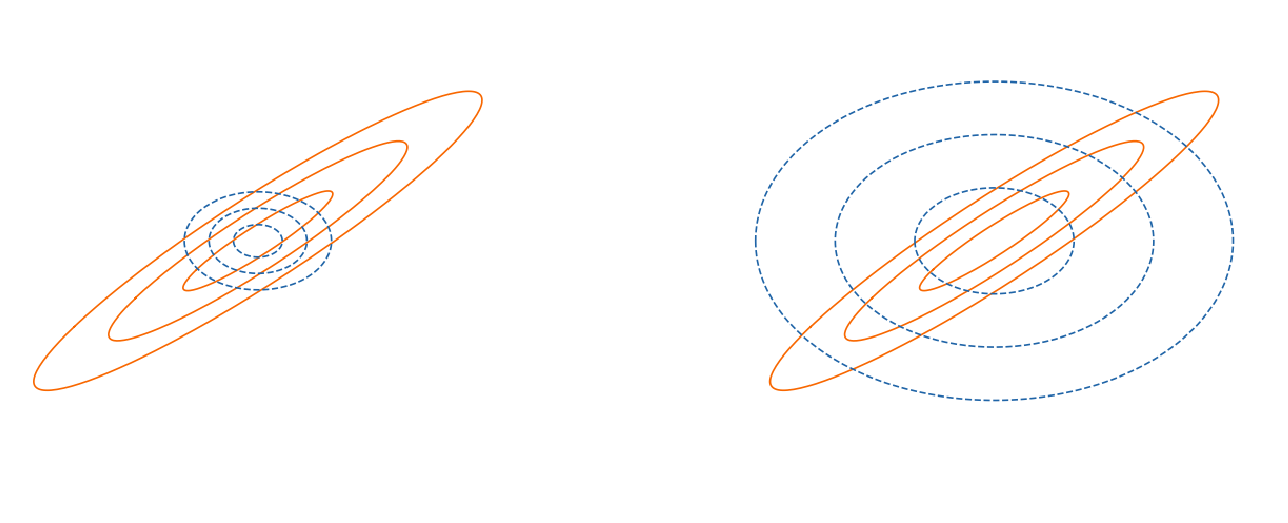
Laplacian approximation

  • left : backward KL DKL(q∥p)D_{KL}(q\Vert p) (blue is qq, orange is pp)
  • right : forward KL DKL(p∥q)D_{KL}(p\Vert q)

ELBO

Q∗=argminQ∈Q DKL(Q(Z)∥P(Z∣X))=argmaxQ∈Q EZ∼Q(Z)[log(P(X∣Z))]−DKL(Q(Z)∣∣P(Z))\begin{aligned} Q^* &= \underset{Q\in\mathcal Q}{argmin}~D_{KL}(Q(Z)\Vert P(Z|X)) \\ &= \underset{Q\in\mathcal Q}{argmax}~\mathbb E_{Z\sim Q(Z)}[log(P(X|Z))] - D_{KL}(Q(Z)||P(Z)) \end{aligned}

Reparameterization tricks

5. Markov Chain Monte Carlo(MCMC)

π=πP\pi = \pi P

where π\pi is the stationary state, PP is the transition matrix

ergodic : ∃t∈N→(P)t>0\exist t\in \mathbb N \rightarrow (P)^t >0

Metropolis-Hastings Algorithm (MH Algorithm)

given proposal distribution R(x′∣x)R(x'|x) and unnormalized stationary distribution Q(x)Q(x)

accpet rate α=min{1,Q(x′)R(x∣x′)Q(x)R(x′∣x)}\alpha = min\{1, \frac{Q(x')R(x|x')}{Q(x)R(x'|x)}\}

new transition matrix col_standarlize(R⊙α)col\_standarlize(R \odot \alpha)

Gibbs Sampling

a special case of MH algorithm, with αij=1\alpha_{ij} = 1

Metropolis Adjusted Langevin Algorithm(MALA)

R(x′∣x)=N(x′∣x−τ∇f(x);2τI)R(x'|x) = \mathcal N(x'|x-\tau \nabla f(x) ;2\tau I)

Stochastic Graident Langevin Dynamics (SGLD)

θt+1=θt−η(∇log p(θt)+Nn∑j=1n∇logp(yij∣θt,xij))+ϵtϵt∼N(0,2ηI)\theta_{t+1} = \theta_t - \eta(\nabla log~p(\theta_t) + \frac{N}{n}\sum_{j=1}^n \nabla log p(y_{i_{j}} | \theta_t, x_{i_j})) + \epsilon_t \quad \epsilon_t \sim \mathcal N(0, 2\eta I)

where L(θt)L(\theta_t) is the likelihood

6. Bayesian Deep Learning

P(y∣x,θ)=N(y;fμ(x,θμ),exp(fσ(x,θσ)))P(y|x,\theta) = \mathcal N(y;f_\mu(x,\theta_\mu),exp(f_\sigma(x,\theta_\sigma)))

θ^=argminθ−lnP(θ)−∑i=1nlnP(yi∣xi,θ)=argminθλ∣∣θ∣∣22+12∑i=1n[1σ(xi;θσ)2∣∣yi−μ(xi;θμ)∣∣2+lnσ(xi;θσ)2]\begin{aligned} \hat \theta &= \underset{\theta}{argmin} - lnP(\theta) - \sum_{i=1}^{n}lnP(y_i|x_i,\theta) \\ &= \underset{\theta}{argmin}\lambda ||\theta||^2_2 +\frac{1}{2}\sum_{i=1}^n\left[\frac{1}{\sigma(x_i;\theta_\sigma)^2}||y_i-\mu(x_i;\theta_\mu)||^2 + ln\sigma(x_i;\theta_\sigma)^2\right] \end{aligned}

Variational Inference (Bayes by Backprop)

argminq∈QKL(q∣∣p(⋅∣y))=argmaxq∈QEθ∼q[lnP(y∣θ)]−KL(q∣∣p(⋅))\underset{q\in \mathcal Q}{argmin} KL(q||p(\cdot | y)) = \underset{q\in \mathcal Q}{argmax}\mathbb E_{\theta\sim q}[lnP(y|\theta)] - KL(q||p(\cdot))

p(⋅)p(\cdot) is posterior for θ\theta here

Evidence Lower Bound (ELBO)

L(q)=Eθ∼q[lnP(y∣θ)]−KL(q∣∣p(⋅))L(q) = \mathbb E_{\theta\sim q}[lnP(y|\theta)] - KL(q||p(\cdot))

Prediction

P(y′∣x′,X,Y)=Eθ∼q[P(y′∣x′,θ)]P(y'|x',X,Y) = \mathbb E_{\theta\sim q}[P(y'|x',\theta)]

Var[y′∣x′,X,Y]=Eθ∼q[Var[y′∣x′,θ]]+Var[E[y′∣x′,θ]]Var[y'|x',X,Y] = {\color{lightblue}\mathbb E_{\theta\sim q}[Var[y'|x',\theta]]}+{\color{orange}Var[\mathbb E[y'|x',\theta]]}

Eθ∼q[Var[y′∣x′,θ]]{\color{lightblue}\mathbb E_{\theta\sim q}[Var[y'|x',\theta]]} : Aleatoric uncertainty(random)

Var[Eθ∼q[y′∣x′,θ]]{\color{orange}Var[\mathbb E_{\theta\sim q}[y'|x',\theta]]} : Epistemic uncertainty(knowledge)

Stochastic Weight Averaging-Gaussian(SWAG)

μSWA=1T∑1TθiΣSWA=1T−1∑1T(θi−μSWA)(θi−μSWA)T\begin{aligned} \mu_{SWA} &= \frac{1}{T}\sum_1^T \theta_i\\ \Sigma_{SWA} &= \frac{1}{T-1}\sum_1^T(\theta_i - \mu_{SWA})(\theta_i-\mu_{SWA})^T \end{aligned}

7. Bayesian Optimization

Uncertainty Sampling

xt=argmaxx∈Dσt−12(x)x_t = \underset{x\in D}{argmax}\sigma_{t-1}^2(x)

  • maximizing information gain in homoscedastic noise case
  • limt→∞ x^t=argmax∈D μt(x)\underset{t\rightarrow \infin}{lim}~\hat x_t = \underset{\in D}{argmax}~\mu_t(x), f(x^)→f(x∗)f(\hat x )\rightarrow f(x^*)

Mutual Information

F(s)=H(f)−H(f∣ys)=12log∣I+σ−2Ks∣F(ST)≥(1−1e)maxS⊆D,∣S∣≤T F(S)F(s) = H(f) - H(f|y_s) = \frac{1}{2}log|I+\sigma^{-2}K_s| \\ F(S_T) \ge (1-\frac{1}{e})\underset{S\subseteq D,|S|\le T}{max}~F(S)

regret

RT=∑t=1T(maxx∈Df(x)−f(xt))R_T = \sum_{t=1}^T (max_{x\in D}f(x)-f(x_t))

sublinear if RTT→0\frac{R_T}{T} \rightarrow 0

Multi-arm bandit

acquisition↑⟺exploitationacquisition↓⟺explorationacquisition\uparrow \Longleftrightarrow exploitation\\ acquisition\downarrow \Longleftrightarrow exploration

Upper Confidence Sampling(UCB)

a=μt(x)+βσt(x)a = \mu_t(x) + \beta \sigma_t(x)

Probability of Improvement(PI)

a=Φ(μt(x)−f∗σt(x))a = \Phi\left(\frac{\mu_t(x)-f^*}{\sigma_t(x)}\right)

Expected Improvement(EI)

a=(μt(x)−f∗)Φ(μt(x)−f∗σt(x))+σt(x)ϕ(μt(x)−f∗σt(x))a = (\mu_t(x)-f^*)\Phi\left(\frac{\mu_t(x)-f^*}{\sigma_t(x)}\right) + \sigma_t(x)\phi\left(\frac{\mu_t(x)-f^*}{\sigma_t(x)}\right)

8. Reinforcement Learning

Bellman Theorem

V∗(x)=maxa(r(x,a)+γ∑x′P(x′∣x,a)V∗(x′))V^*(x) = max_a(r(x,a) + \gamma\sum_{x'}P(x'|x,a)V^*(x'))

Hoffeding bound

P(∣μ−1n∑i=1nZi∣>ε)≤2exp(−2nε2C2)P(|\mu - \frac{1}{n}\sum_{i=1}^n Z_i|>\varepsilon) \leq 2exp(-\frac{2n\varepsilon^2}{C^2})

model-based RL

learn Markov Decision Processes, learn pp and rr, e.g gaussian process

model-free RL

learn value function directly

on policy

model has control of the action

off policy

Value Iteration

polynomial time, performance depend on the input

  • guarantee converge to an ε\varepsilon optimal policy not the exact optimal policy

Policy Iteration

  • guaranteed to monotonically improve the policy

ϵ\boldsymbol \epsilon greedy Algorithm

model-based

when random number <ϵ<\epsilon do the random action

R~max~ algorithm

model-based

set reward RR and transition probability P(x∗∣x,a)=1P(x^*|x,a)=1 at first

  • with probability 1−σ1-\sigma, R~max~ will reach an ε\varepsilon - optimal
  • polynomial time in ∣X∣,∣A∣,T,1ε,log(1δ)|X|, |A|, T,\frac{1}{\varepsilon},log(\frac{1}{\delta})

Temporal Difference(TD) - Learning

model-free

on policy

V^π(x)←(1−αt)V^π(x)+αt(r+γV^π(x′))\hat V^\pi (x)\leftarrow (1-\alpha_t)\hat V^\pi (x) + \alpha_t(r+\gamma\hat V^\pi (x'))

Theorem ∑tαt=∞,∑tαt2<∞⇒P(V^π→Vπ)=1\sum_t\alpha_t=\infin,\sum_t\alpha_t^2 < \infin \Rightarrow P(\hat V^\pi\rightarrow V^\pi) = 1

Q-Learning

model-free: estimate Q∗Q^* directly from samples,

off policy

Q^∗←(1−αt)Q^∗(x,a)+αt(r+γmaxa′Q^∗(x′,a′))\hat Q^* \leftarrow (1-\alpha_t)\hat Q^*(x,a) + \alpha_t(r+\gamma \underset{a'}{max}\hat Q^*(x',a'))

Init: Q^∗(x,a)=Rmax1−γΠt=1Tinit(1−αt)−1\hat Q^*(x,a) = \frac{R_{max}}{1-\gamma}\Pi_{t=1}^{T_{init}}(1-\alpha_t)^{-1}

Theorem ∑tαt=∞,∑tαt2<∞⇒P(Q^∗→Q∗)=1\sum_t\alpha_t=\infin,\sum_t\alpha_t^2 < \infin \Rightarrow P(\hat Q^*\rightarrow Q^*) = 1

  • with probability 1−σ1-\sigma, R~max~ will reach an ε\varepsilon - optimal
  • polynomial time in ∣X∣,∣A∣,T,1ε,log(1δ)|X|, |A|, T,\frac{1}{\varepsilon},log(\frac{1}{\delta})
  • need decay learning rate to guarantee convergence

DQN

L(θ)=∑(r+γmaxa′Q(x′,a′;θold)−Q(x,a;θ))2L(\theta) = \sum(r + \gamma\underset{a'}{max}Q(x',a';\theta^{old})-Q(x,a;\theta))^2

problem : maximization bias

Double DQN

L(θ)=∑(rt+γQ(xt+1,argmaxa′Q′(x,a;θ′);θ)−Q(x,a;θ))2L(\theta) = \sum(r_t + \gamma Q(x_{t+1}, \underset{a'}{argmax}Q'(x,a;\theta');\theta)-Q(x,a;\theta))^2

θ′←τθ+(1−τ)θ′\theta' \leftarrow \tau \theta + (1-\tau)\theta'

Policy Gradient

model free

J(θ)=Eτ∼πθ(τ)r(τ)J(\theta) = \mathbb E_{\tau\sim \pi_\theta(\tau)}r(\tau)

∇J(θ)=E(x,a)∼πθ[Q(x,a)∇logπ(a∣x;θ)]\nabla J(\theta) = \mathbb E_{(x,a)\sim \pi_\theta}[Q(x,a)\nabla log \pi(a|x;\theta)]

REINFORCE

on policy

∇θJ(θ)=Eτ∼pθ(τ)[∑t=0Tγt(∑t′=tTγt′−trt)∇θlnπθ(at∣xt)]θ←θ+ηt∇θJ(θ)\begin{aligned} \nabla_{\theta} J(\theta) &= \mathbb E_{\tau\sim p_\theta(\tau)}[\sum_{t=0}^T\gamma^t(\sum_{t'=t}^T\gamma^{t'-t}r_t)\nabla_\theta ln\pi_\theta(a_t|x_t)] \\ \theta &\leftarrow \theta + \eta_t \nabla_\theta J(\theta) \end{aligned}

Actor-Critic

on policy

∇θπJ(θπ)=E(x,a)∼πθπ[QθQ(x,a)∇θπlnπθπ(a∣x)]θπ←θπ+ηt∇θπJ(θπ)θQ←θQ−ηt(QθQ(x,a)−r−γQθQ(x′,πθπ(x′)))∇θQQθQ(x,a)\begin{aligned} \nabla_{\theta_\pi} J(\theta_\pi) &= \mathbb E_{(x,a)\sim \pi_{\theta_\pi}} [Q_{\theta_Q}(x,a)\nabla_{\theta_\pi}ln\pi_{\theta_\pi}(a|x)] \\ \theta_\pi &\leftarrow \theta_\pi + \eta_t \nabla_{\theta_\pi}J(\theta_\pi) \\ \theta_Q &\leftarrow \theta_Q - \eta_t(Q_{\theta_Q}(x,a) - r - \gamma Q_{\theta_Q}(x',\pi_{\theta_\pi}(x')))\nabla_{\theta_Q}Q_{\theta_Q}(x,a) \end{aligned}

use baseline to reduce variance

Trust- regin policy optimization (TRPO)

on policy

Proximal Policy Optimization (PPO)

on policy

Lθk(θk)=Eτ∼πk∑t=0∞[πθ(a∣x)πθk(a∣x)(r+γQπθk(x′,a)−Qπθk(x,a))]θk←θk−ηt∇θkLθk(θk)L_{\theta_k}(\theta_k) = \mathbb E{\tau \sim \pi_k}\sum_{t=0}^\infin[\frac{\pi_\theta(a_|x)}{\pi_{\theta_k}(a|x)}(r + \gamma Q^{\pi_{\theta_k}}(x',a)-Q^{\pi_{\theta_k}}(x,a))] \\ \theta_k \leftarrow \theta_k - \eta_t \nabla_{\theta_k}L_{ \theta_k}(\theta_k)

Deep Deterministic Policy Gradients(DDPG)

off policy

randomly add noise the ensure sufficient exploration

θQ←θQ−η∇θQEτ∼πθπ[(QθQ(x,a)−(r+γQθQold(x′,πθπold(x′)))2]θπ←θπ+η∇θπEτ∼πθπ[QθQ(x,πθπ(x))]θQold←(1−ρ)θQold+ρθQθπold←(1−ρ)θπold+ρθπ\begin{aligned} \theta_Q &\leftarrow \theta_Q - \eta \nabla_{\theta_Q} \mathbb E_{\tau\sim\pi_{\theta_\pi}}[(Q_{\theta_Q}(x, a)-(r + \gamma Q_{\theta_Q^{old}}(x',\pi_{\theta_\pi^{old}}(x')))^2] \\ \theta_\pi &\leftarrow \theta_\pi + \eta \nabla_{\theta_\pi} \mathbb E_{\tau\sim\pi_{\theta_\pi}}[Q_{\theta_Q}(x,\pi_{\theta_\pi}(x))] \\ \theta_Q^{old} &\leftarrow (1-\rho)\theta_Q^{old} + \rho \theta_Q \\ \theta_\pi^{old} &\leftarrow(1-\rho)\theta_\pi^{old} + \rho \theta_\pi \end{aligned}

Soft Actor Critic(SAC)

off policy

Random Shooting methods

Monte-Carlo Tree Search


Probabilitisc Artificial Intelligence
https://walkerchi.github.io/2023/02/02/ETHz/ETHz-PAI/
Author
walkerchi
Posted on
February 2, 2023
Licensed under